Workshop
Workshop program and overall results
Workshop
The SPEAR Challenge Workshop was held online on Thursday 30th of March. Below you can find videos of the presentations and a summary of the results.
Programme
UK time (BST)
Session 1 (3:00 pm - 4:15 pm)
- 3:00 pm Welcome & Introduction to the SPEAR Challenge
- 3:30 pm Zhongweiyang Xu (Univeristy of Illinois) (paper)
- 3:45 pm Benjamin Stahl (IEM, Gratz) (paper)
-
4:00 pm Iko Pieper (audifon) (paper)
- 4:15 Break (15 min)
Session 2 (4:30 pm - 5:45 pm)
- 4:30pm Invited talk: Augmented audio at Meta and the future of human communication: Technology, challenges, and opportunities
- 5:00 pm Evaluation & results
- 5:30 pm Q&A
- 5:45 pm Wrap up
Results
Teams
Results are presented using the annoymised algorithm labels. The teams contributing each algorithm are given in the table below.
| ID | Team name | Algorithm name | Affiliation | Description |
|---|---|---|---|---|
| alg_A | - | passthrough | - | |
| alg_B | - | baseline | - | |
| alg_C | audifon | aud-1 | audifon GmbH & Co. KG | paper |
| alg_D | audifon | aud-2 | audifon GmbH & Co. KG | paper |
| alg_E | IEM | iem | University of Music and Performing Arts Graz | paper |
| alg_F | IIPHIS | iip-1 | Sogang University | paper |
| alg_G | IIPHIS | iip-2 | Sogang University | paper |
| alg_H | IIPHIS | iip-3 | Sogang University | paper |
| alg_I | IIPHIS | iip-4 | Sogang University | paper |
| alg_J | UIUC | uiuc-1 | Univeristy of Illinois | paper |
| alg_K | UIUC | uiuc-2 | Univeristy of Illinois | paper |
| alg_L | UIUC | uiuc-3 | Univeristy of Illinois | paper |
| alg_M | UIUC | uiuc-4 | Univeristy of Illinois | paper |
| alg_N | UIUC | uiuc-5 | Univeristy of Illinois | paper |
| alg_O | ICL | icl-1 | Imperial College London | |
| alg_P | ICL | icl-2 | Imperial College London |
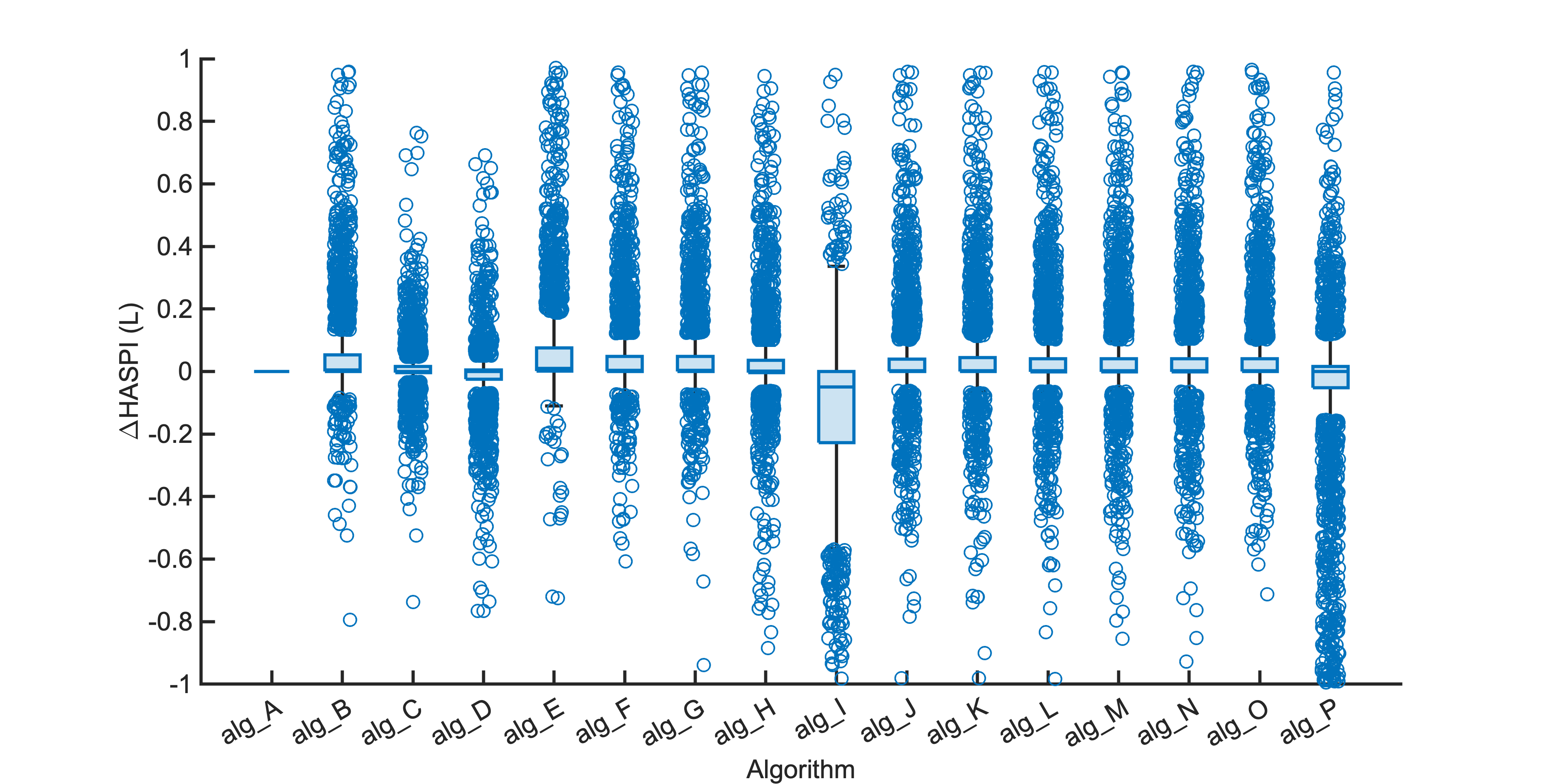
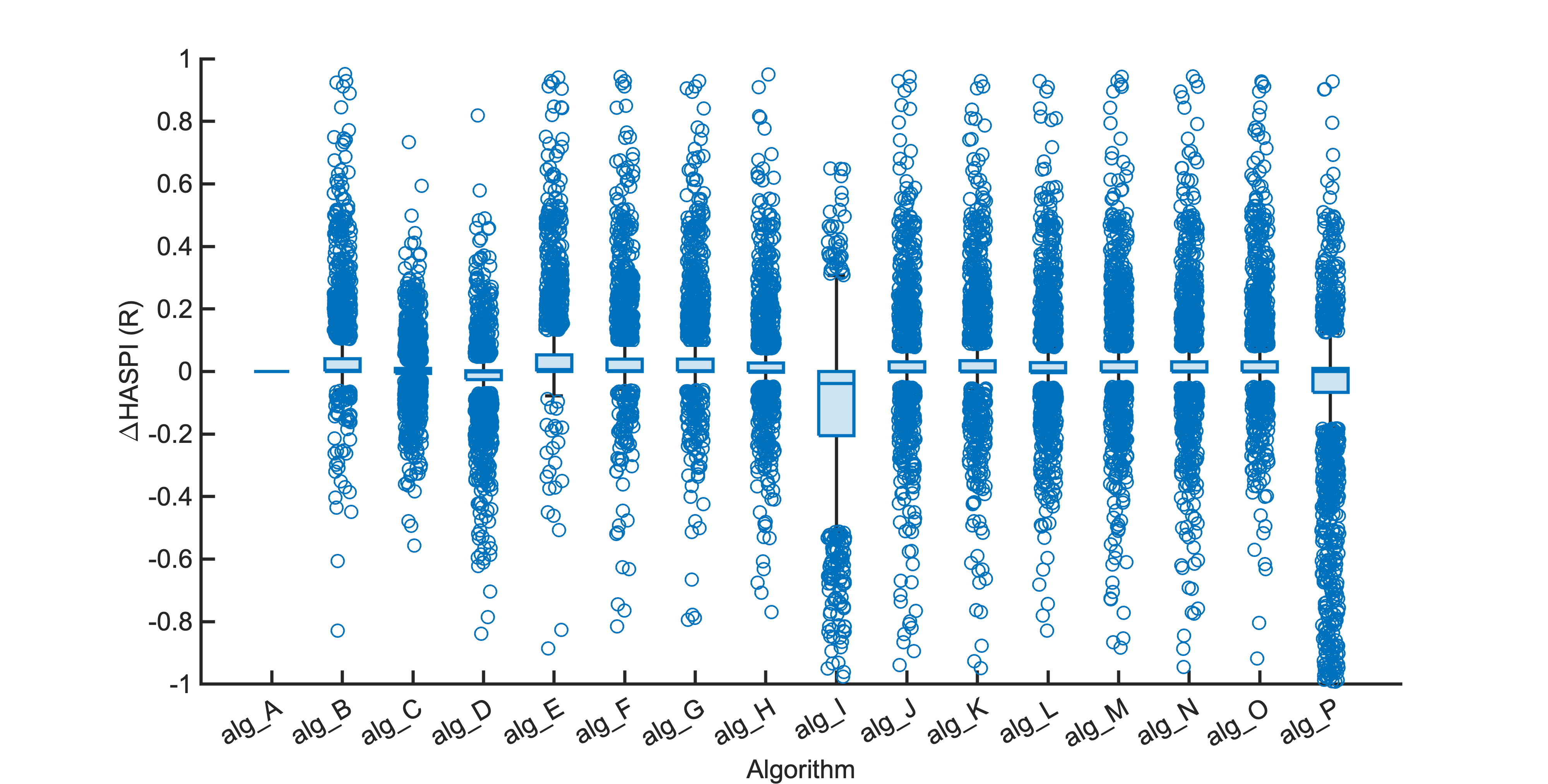
Metrics
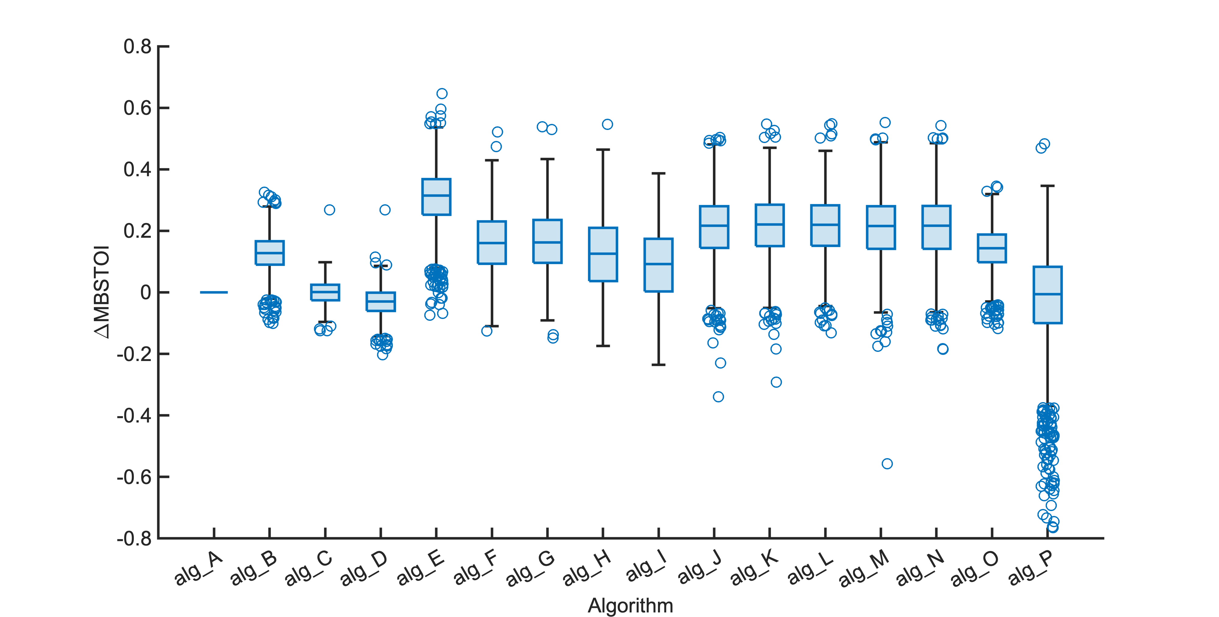
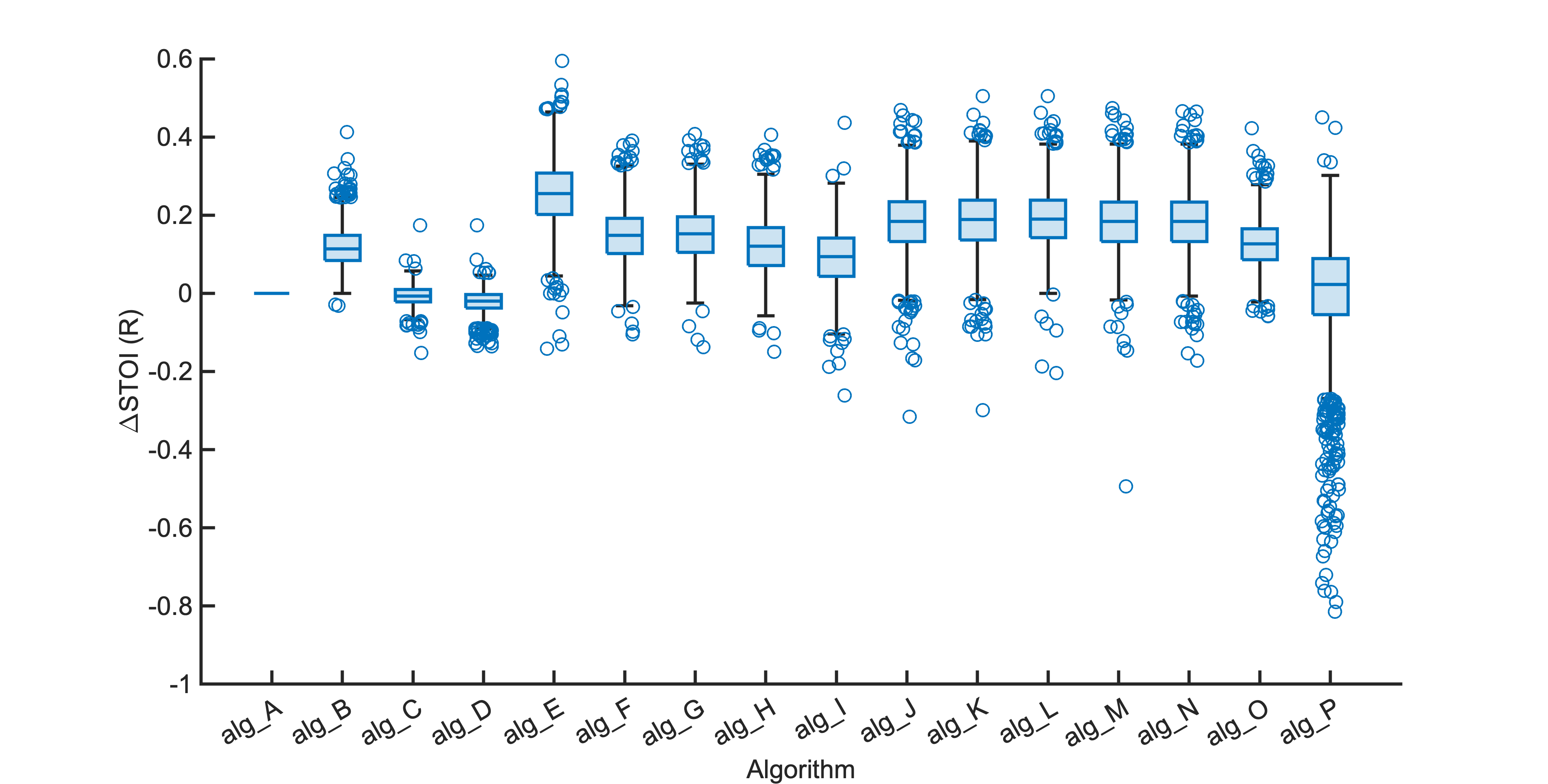
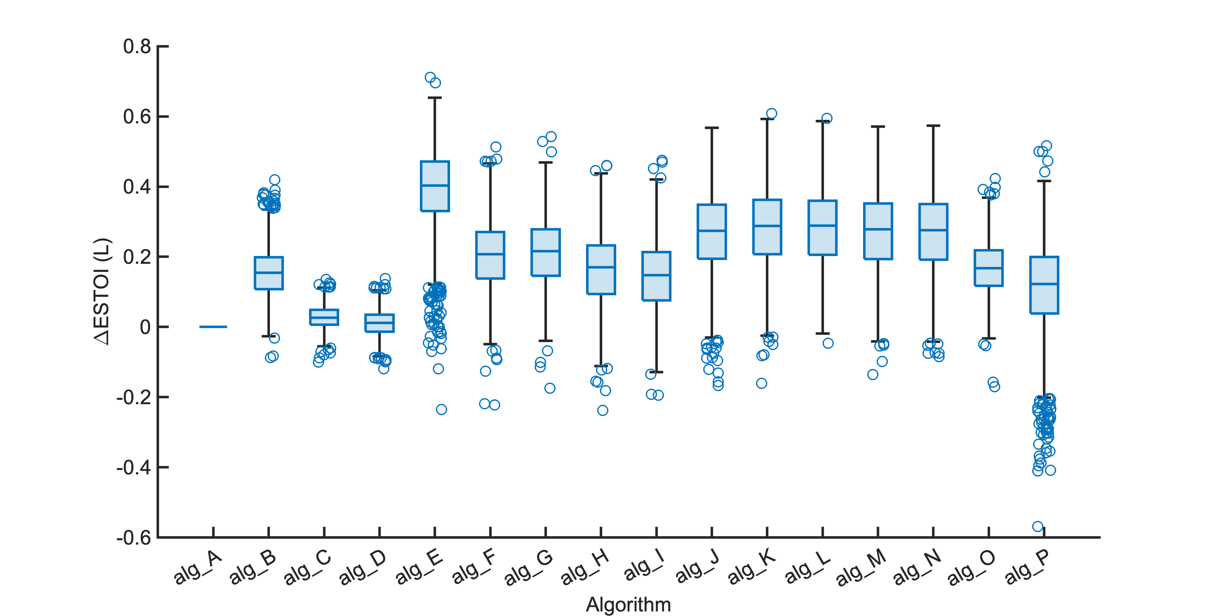
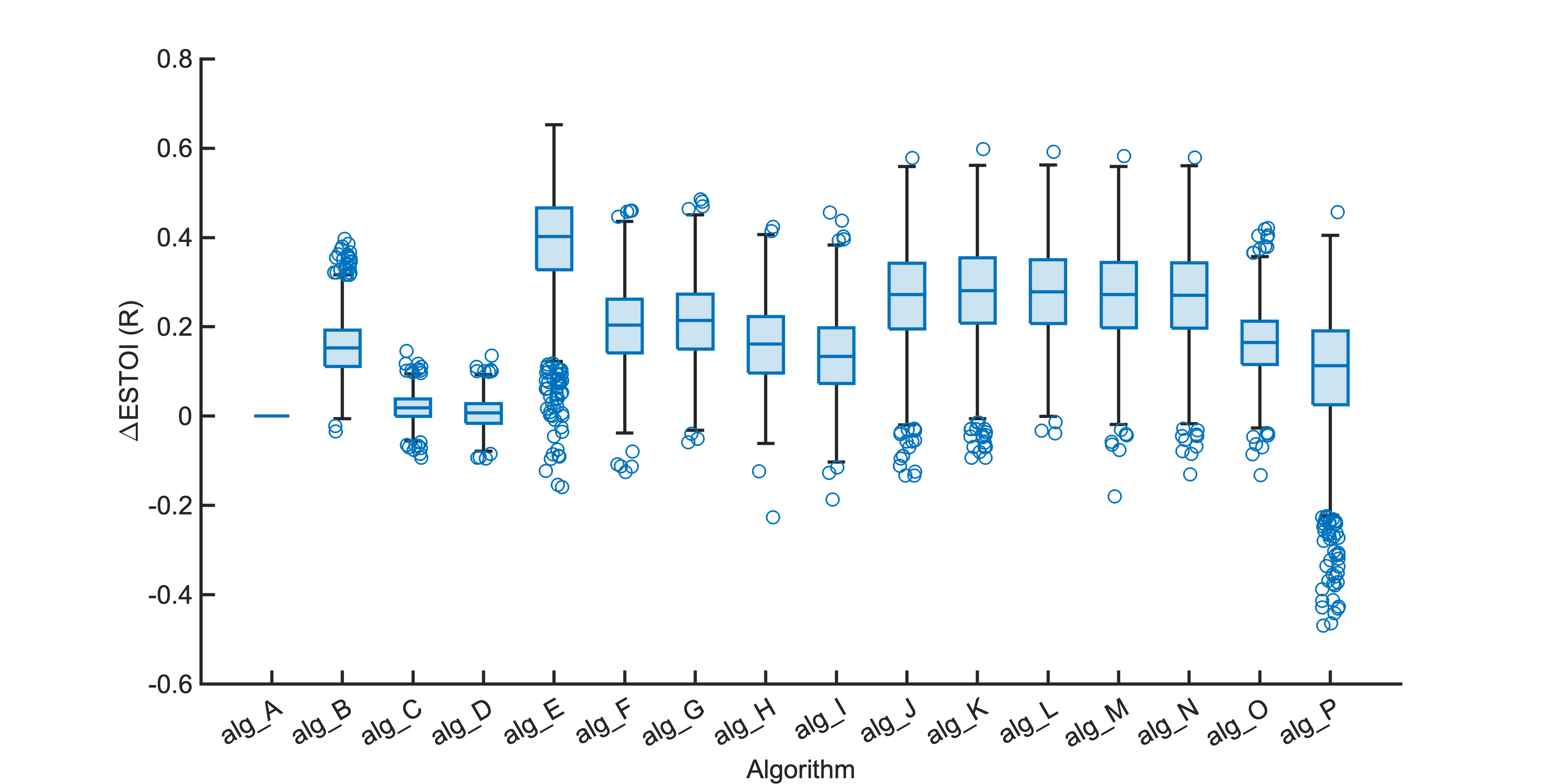
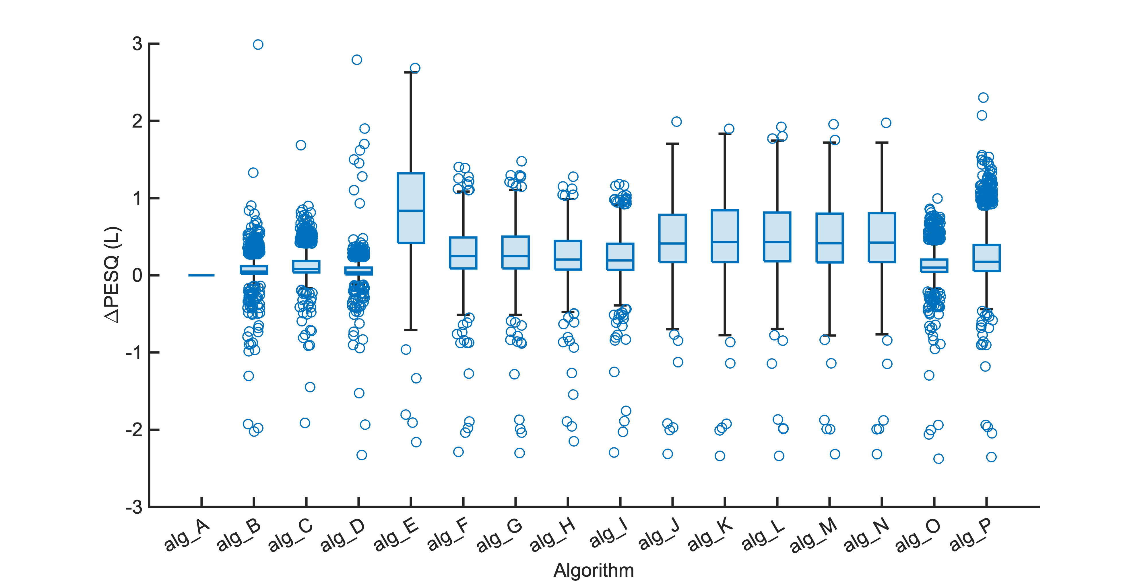
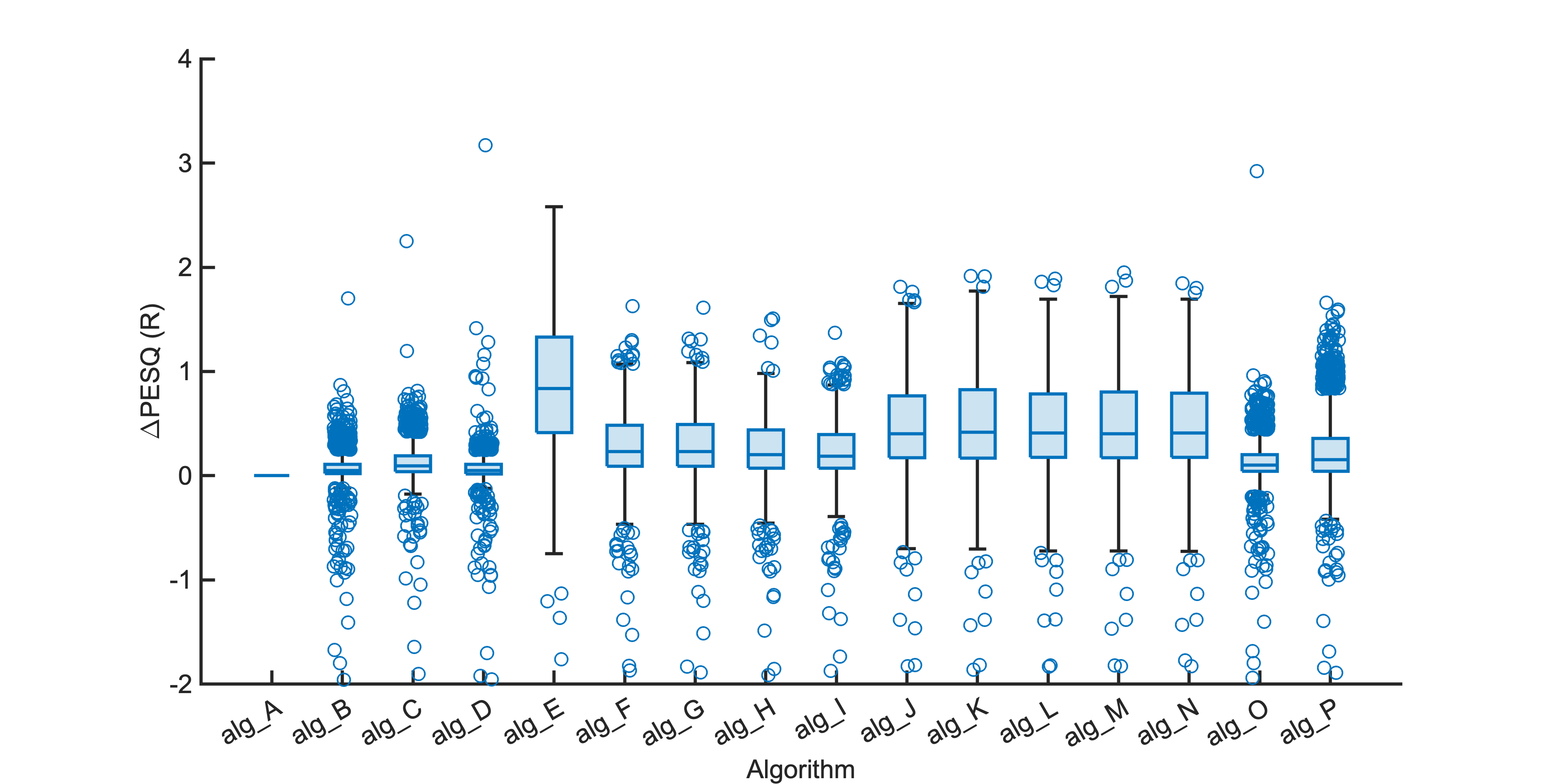
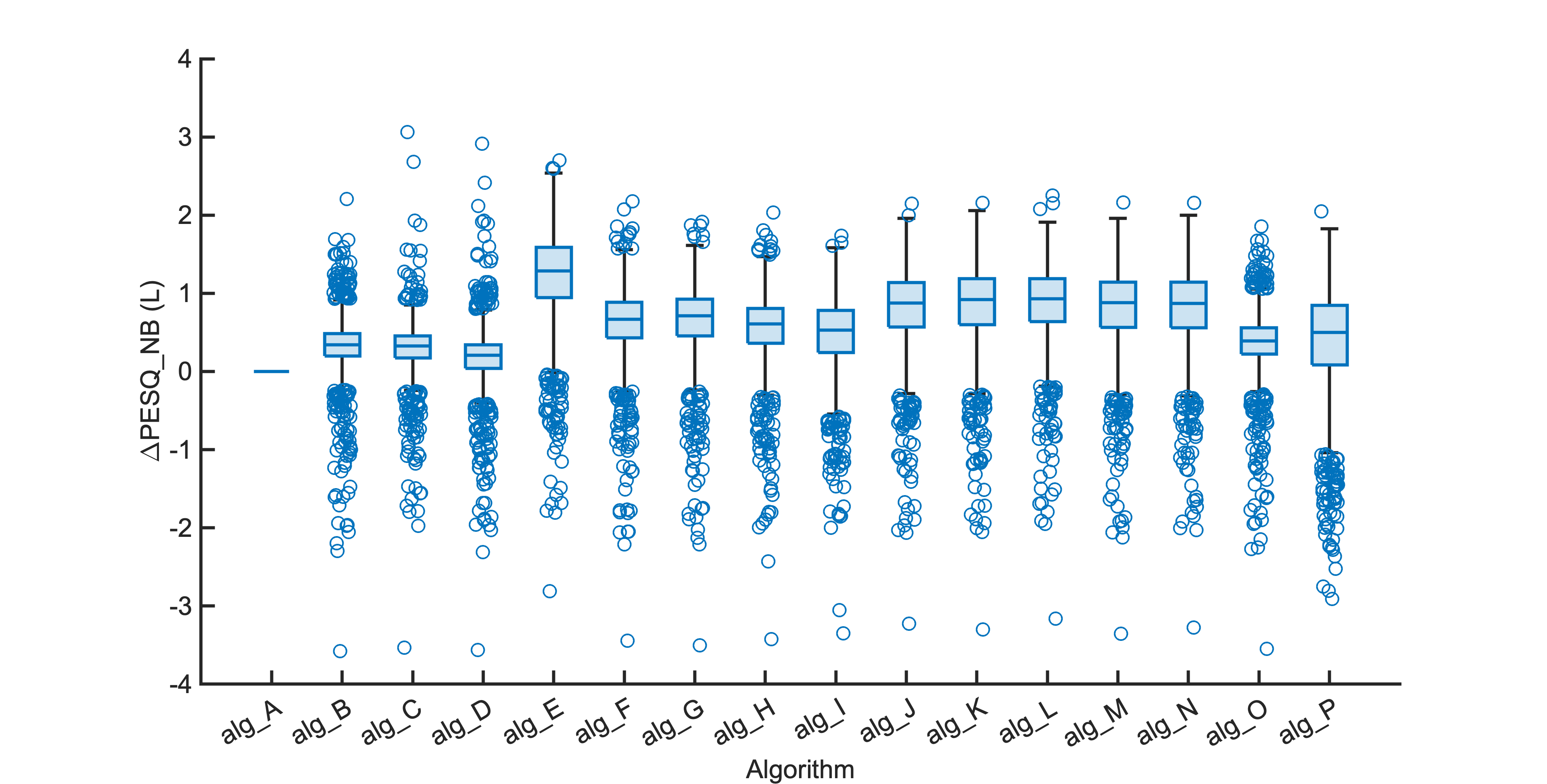
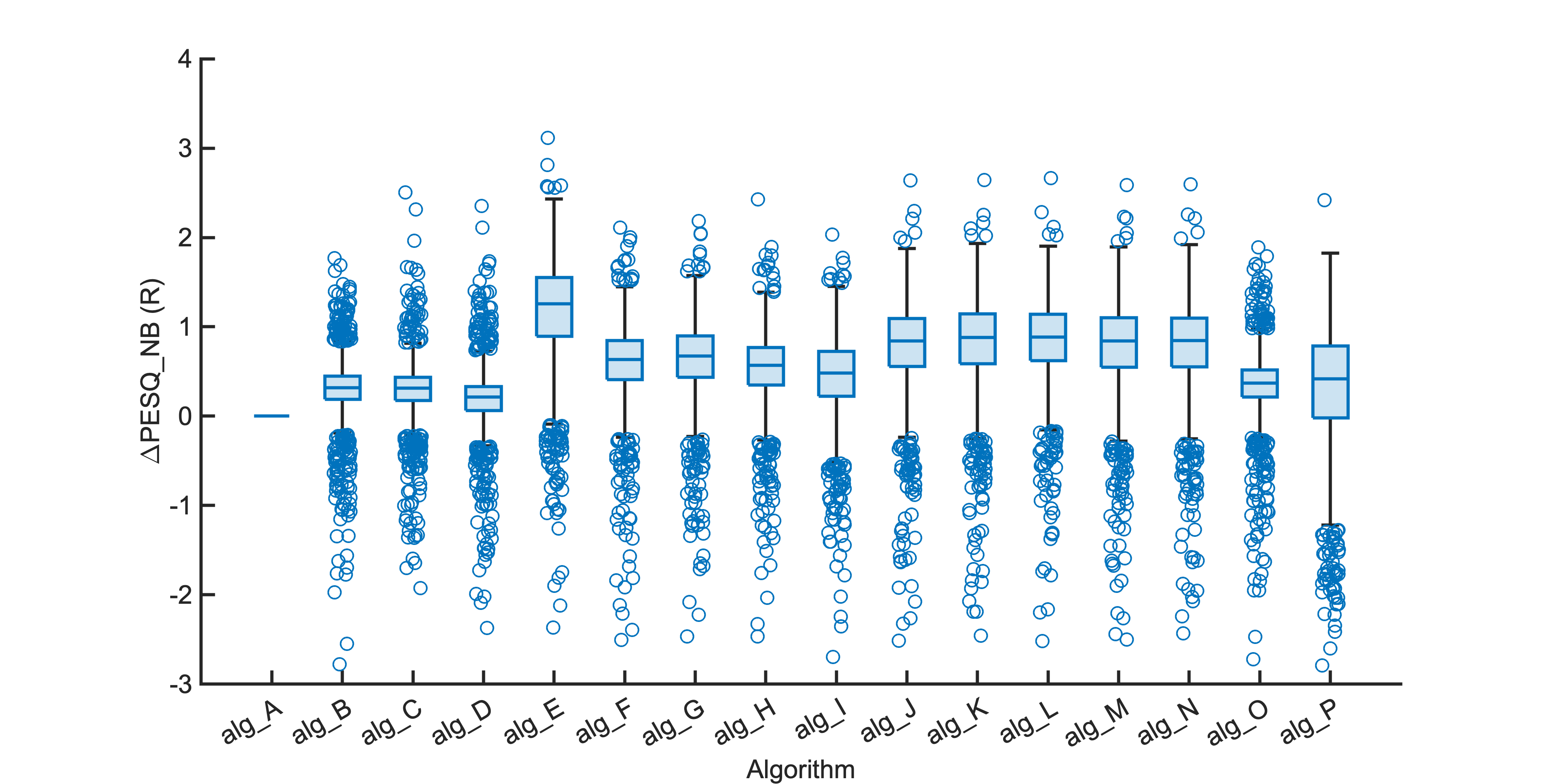
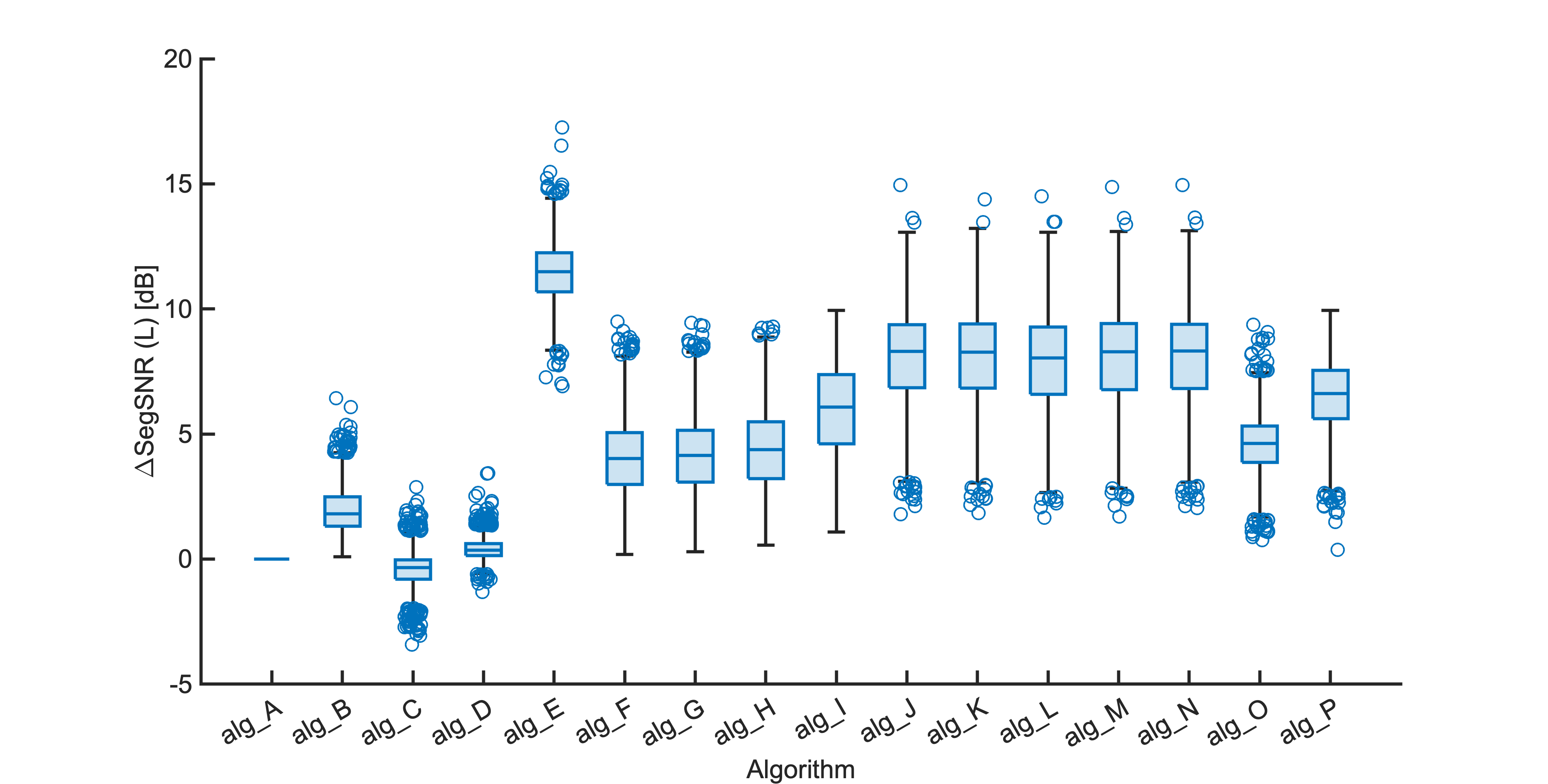
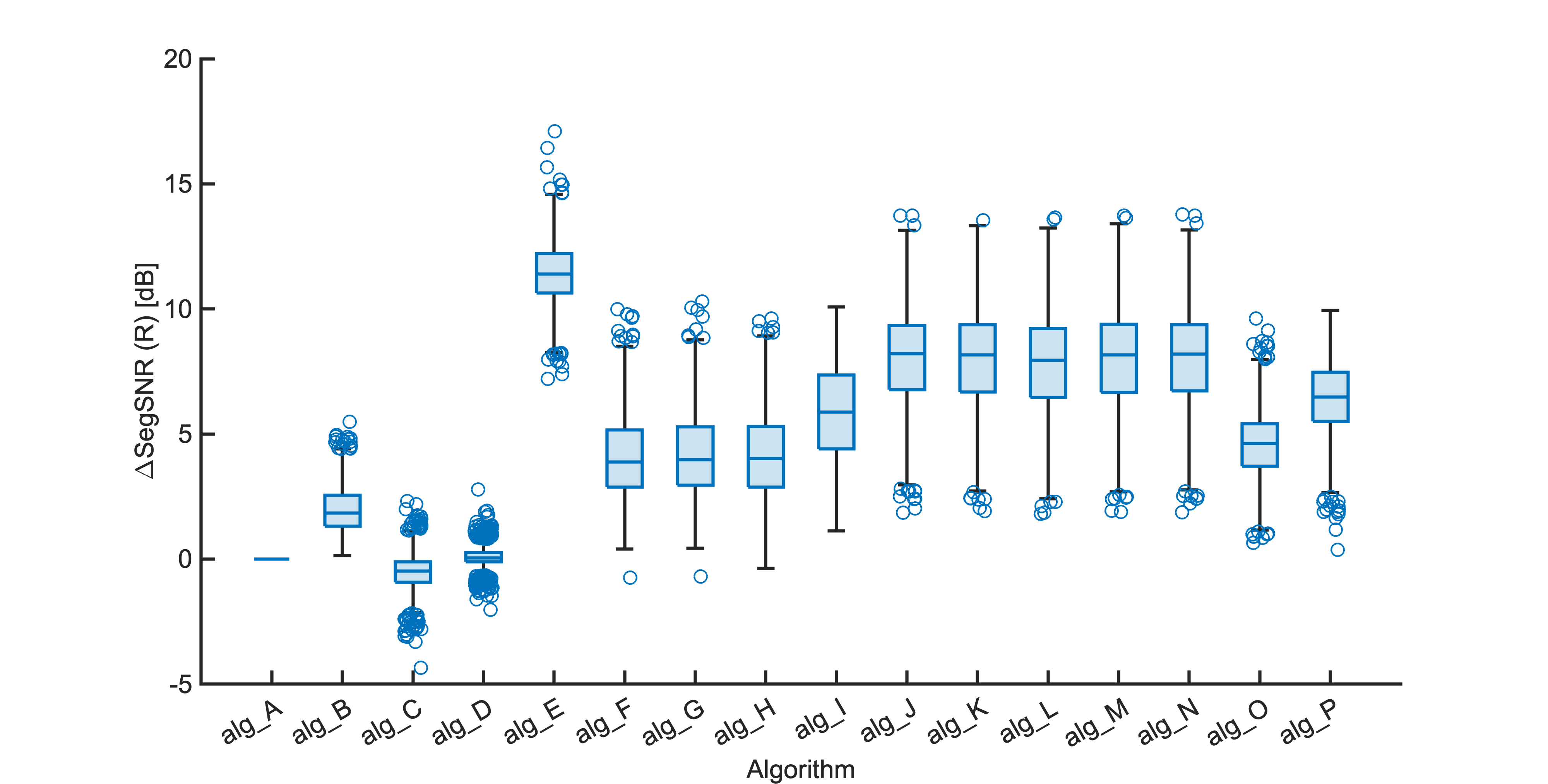
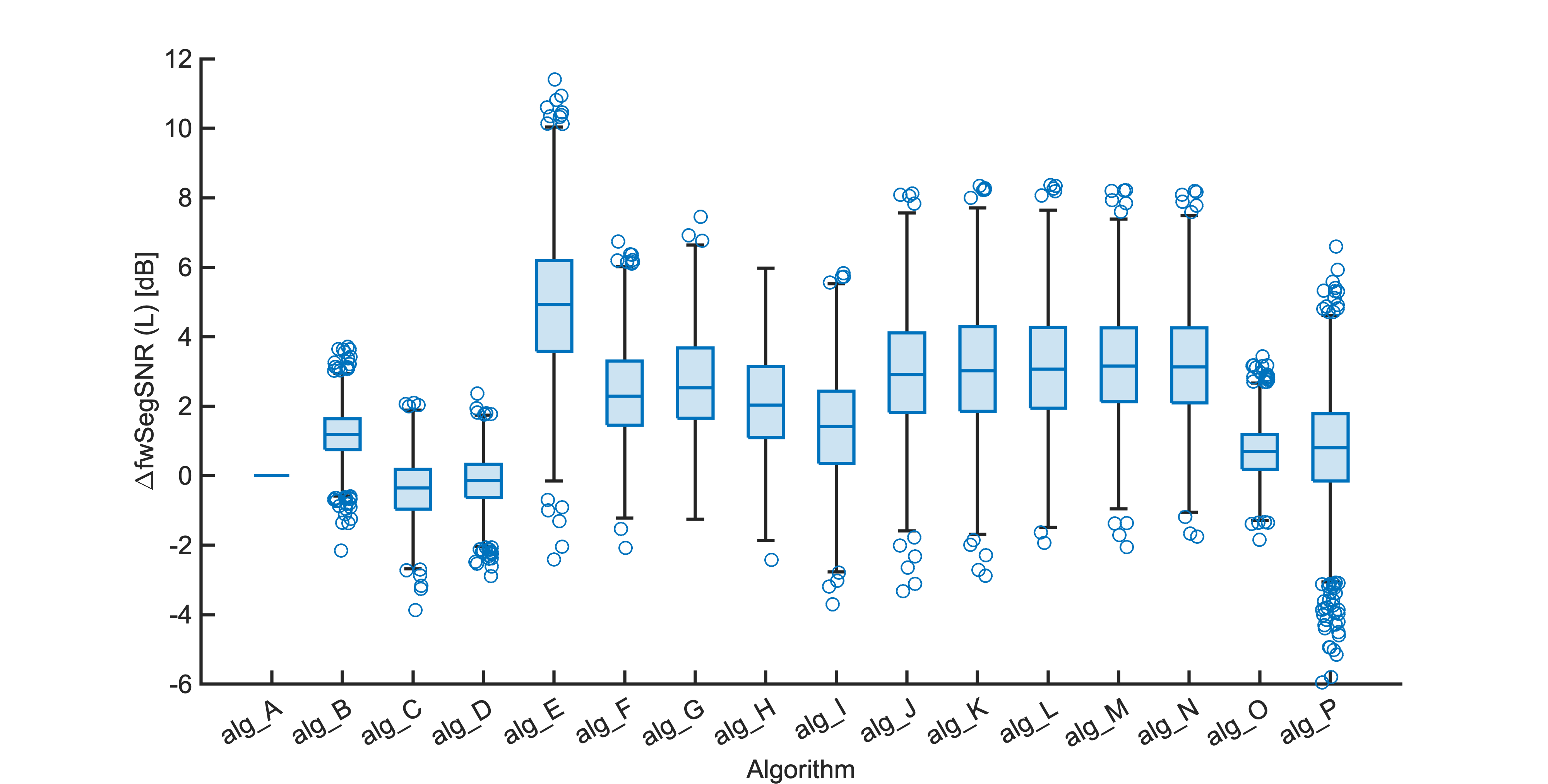
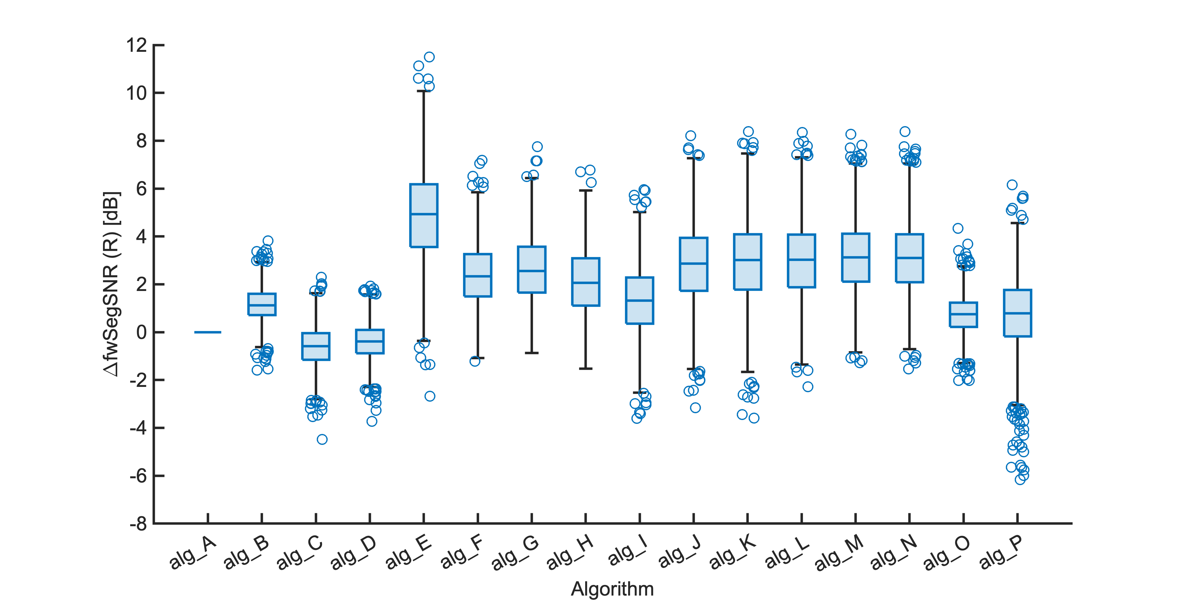
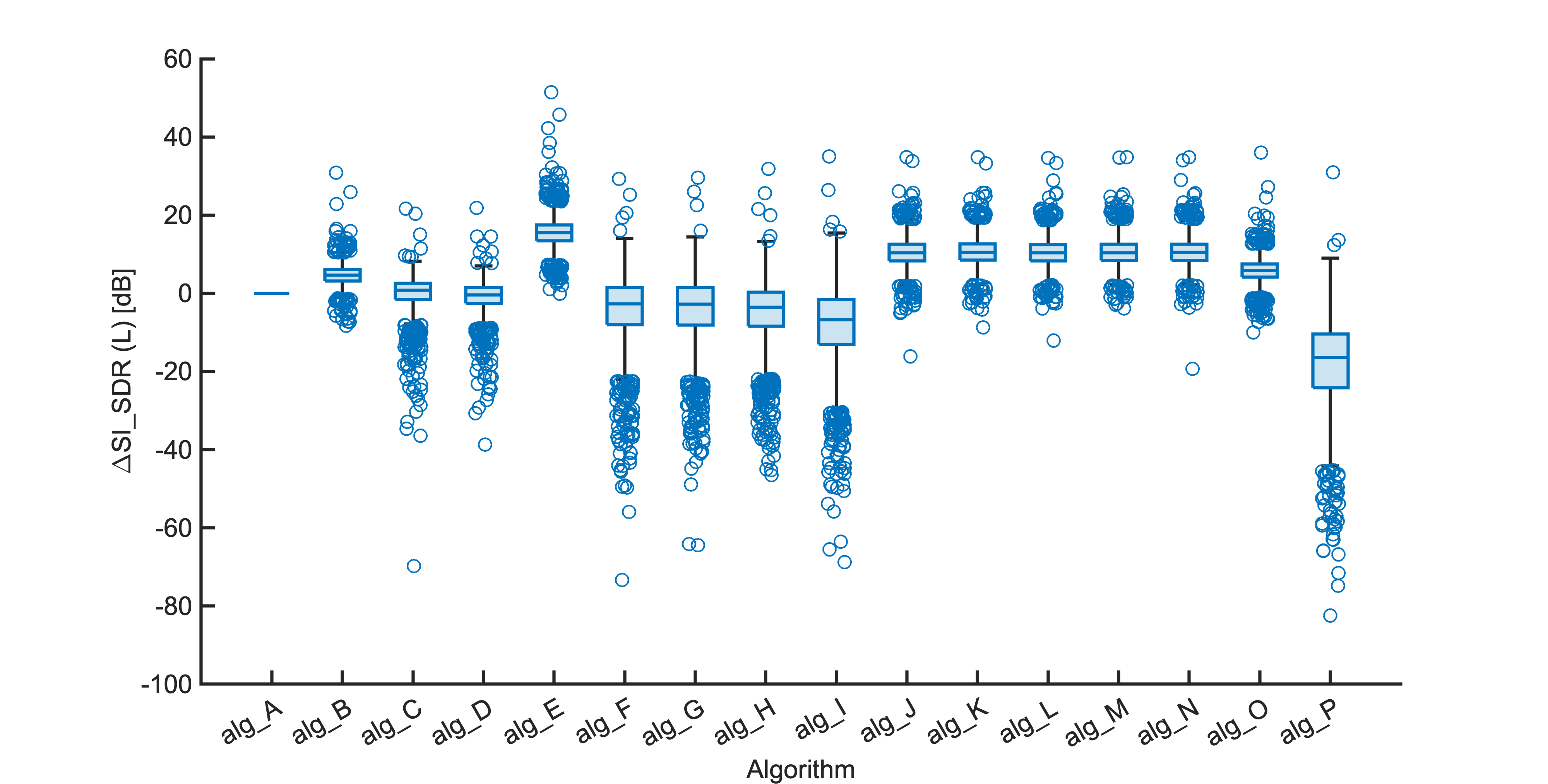
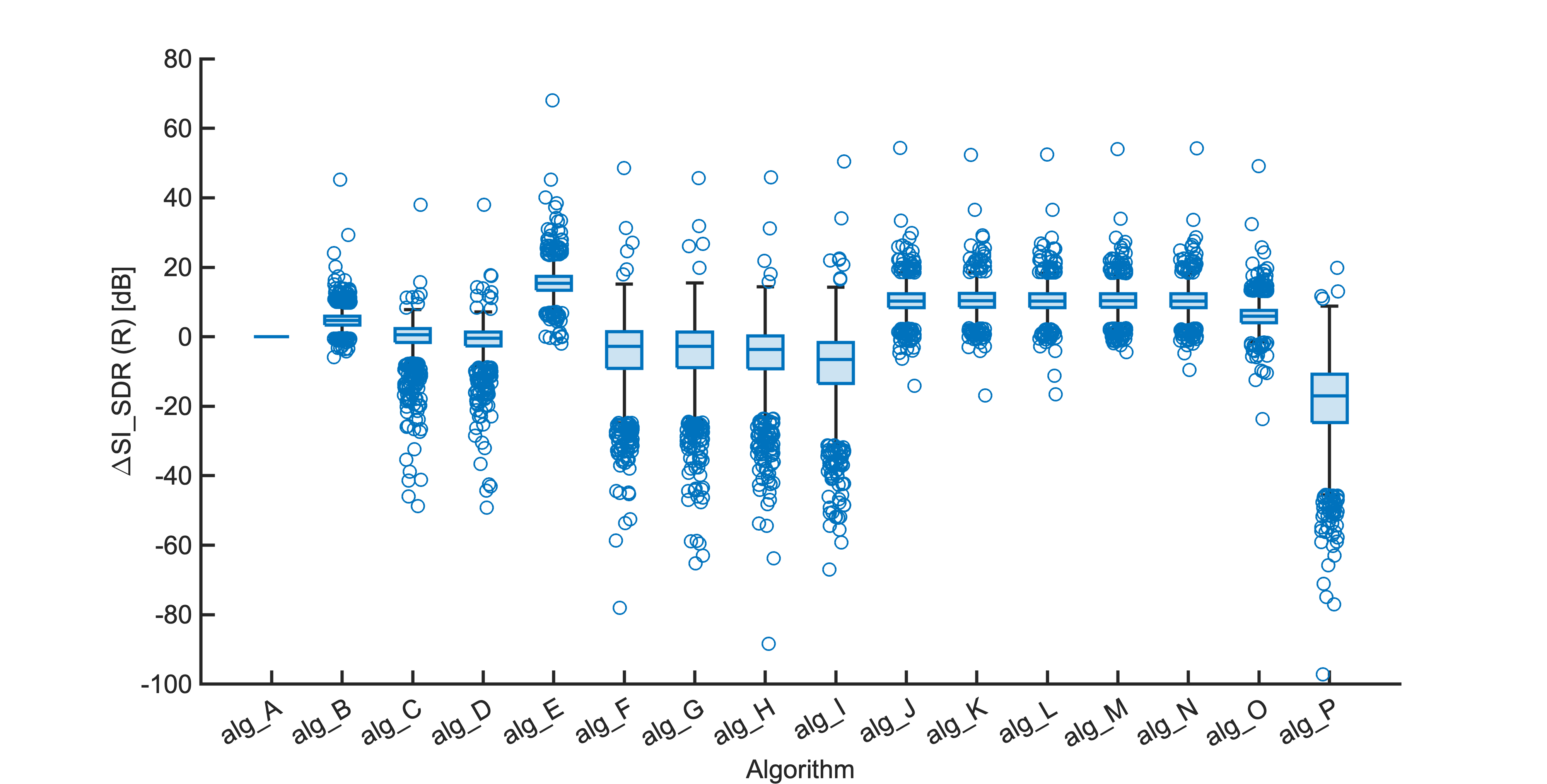
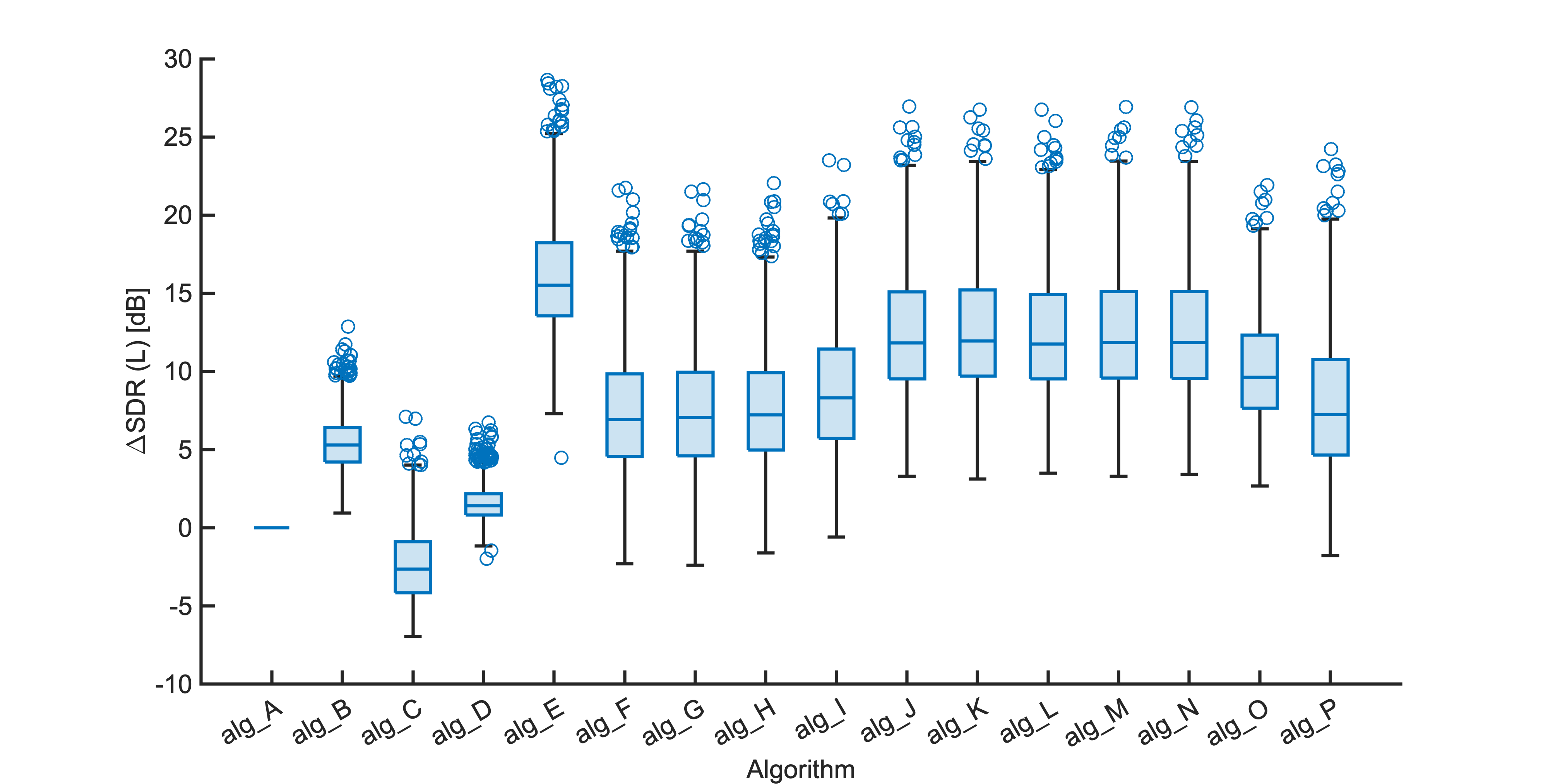
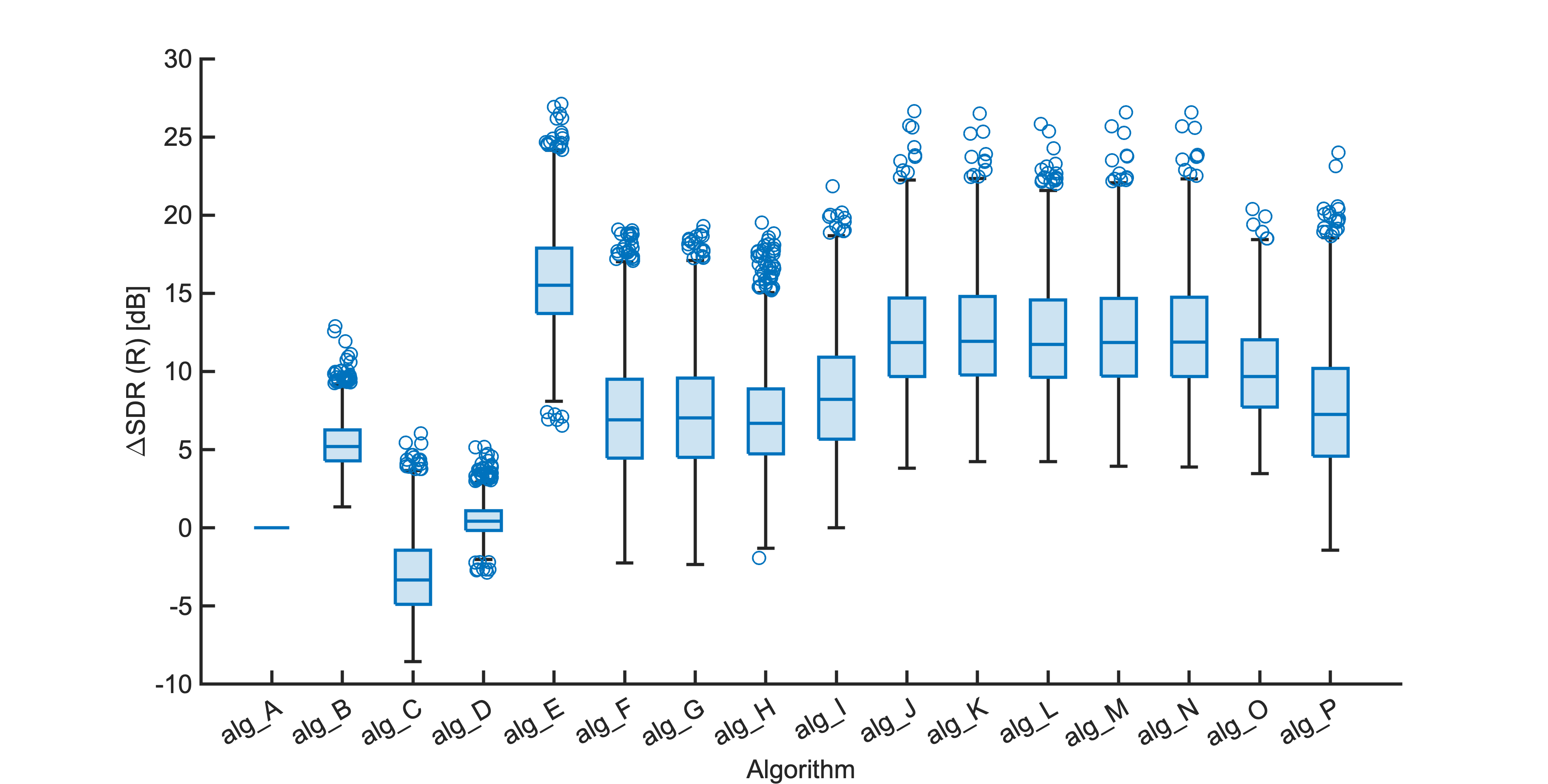
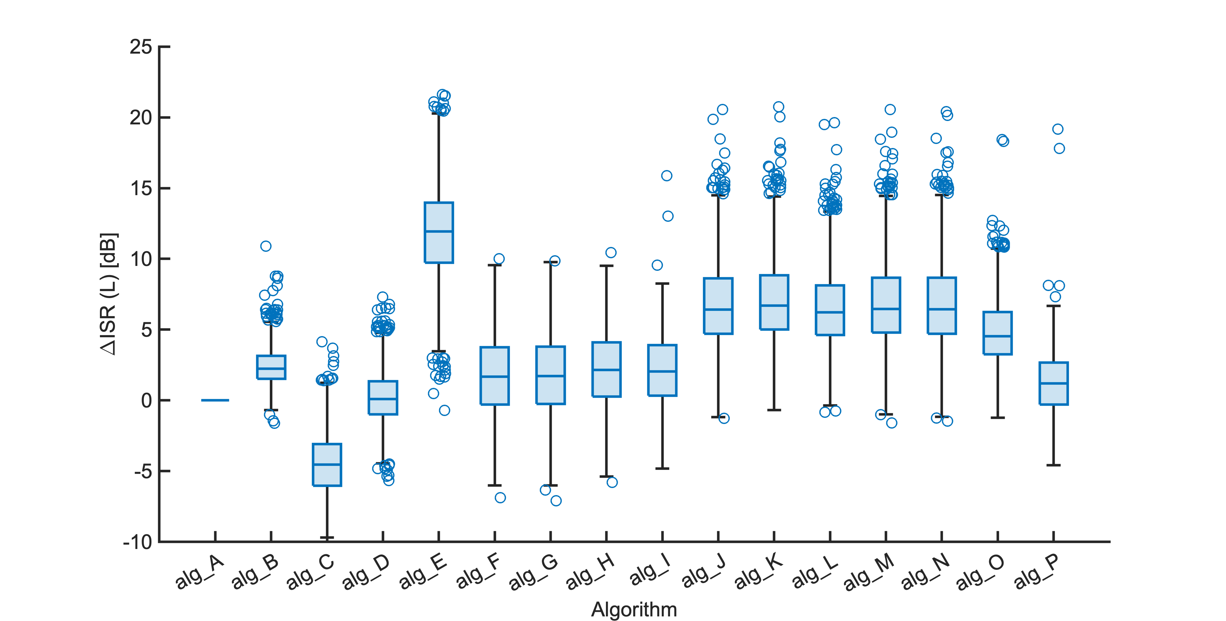
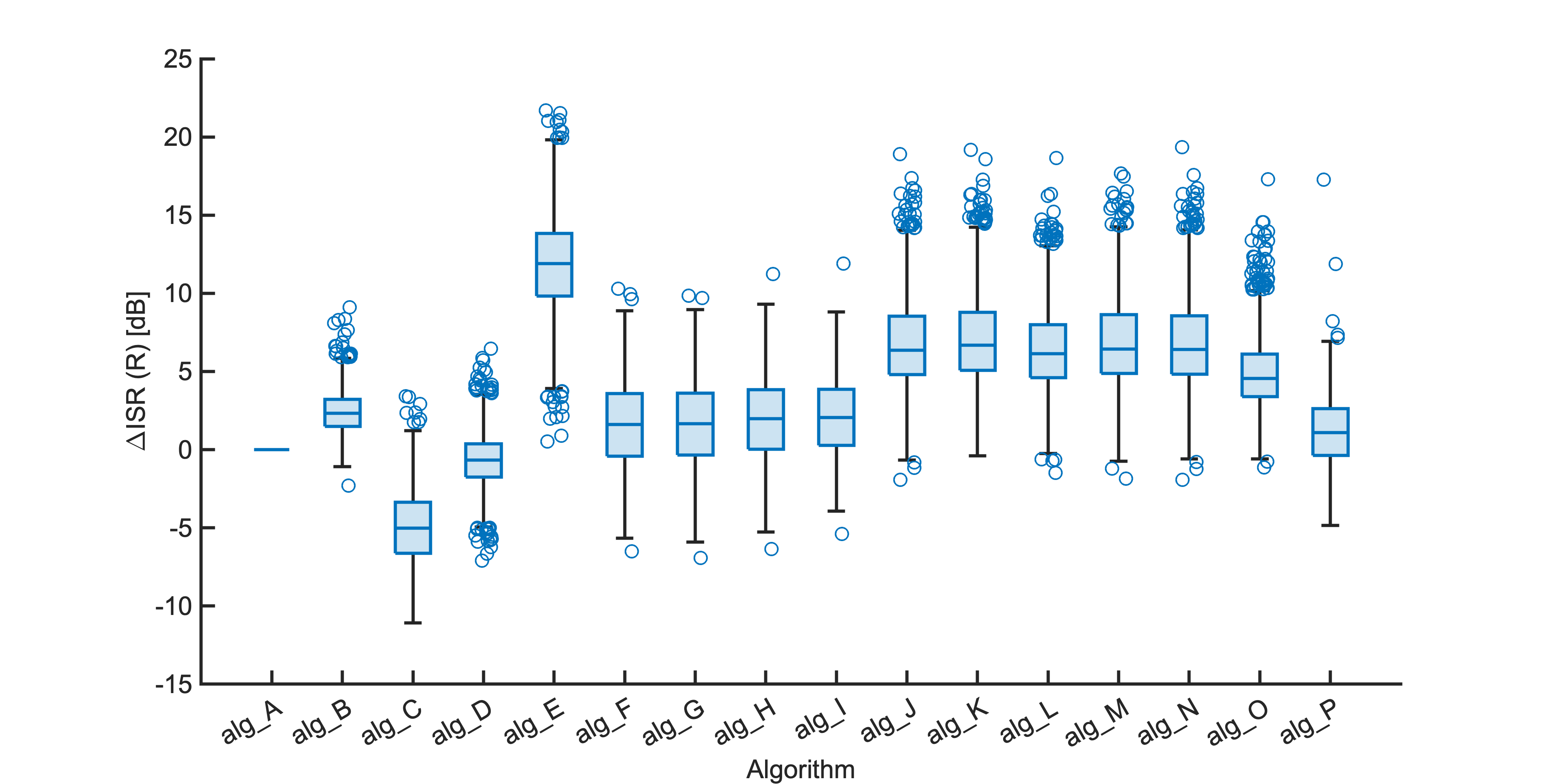
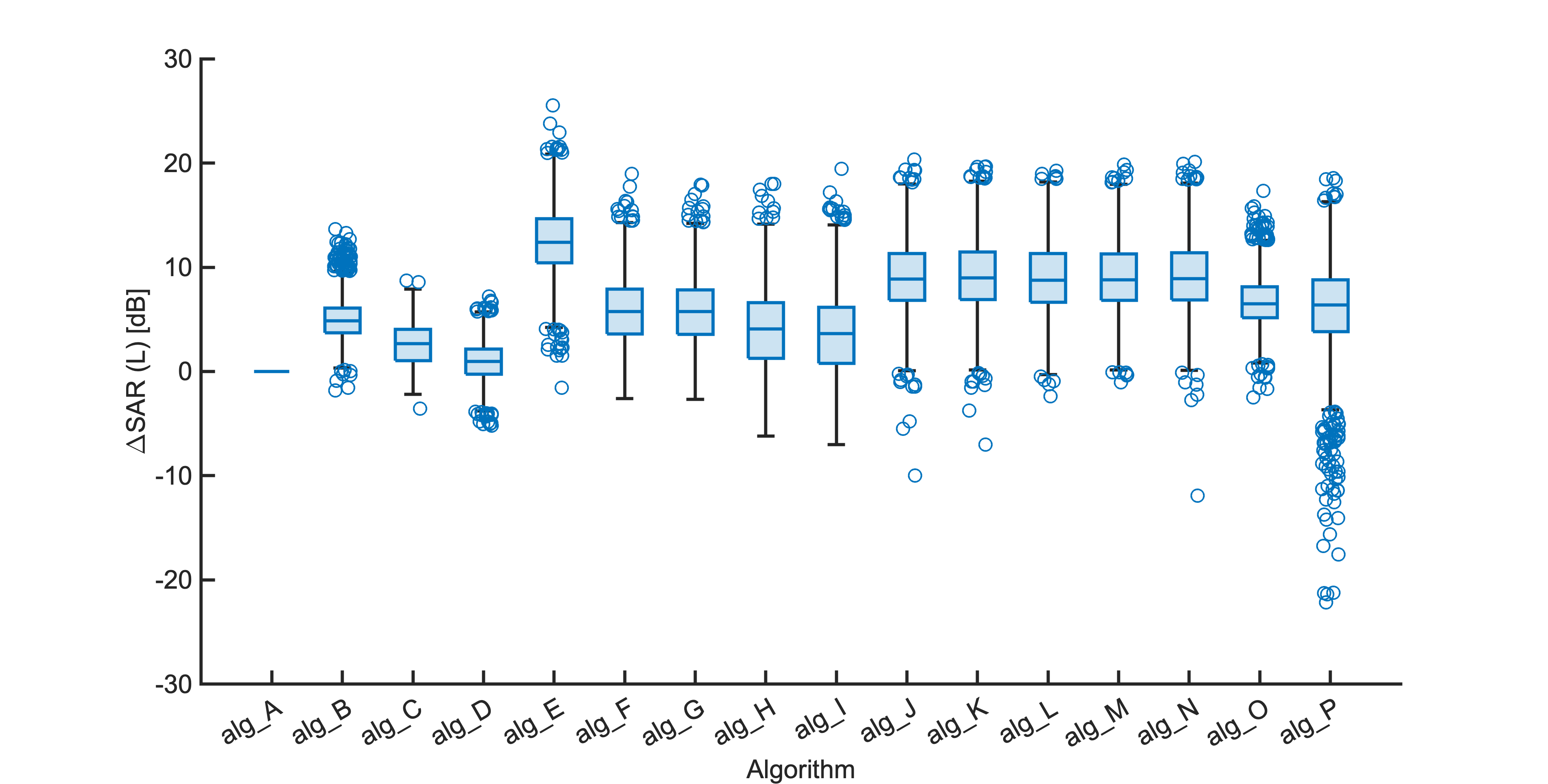
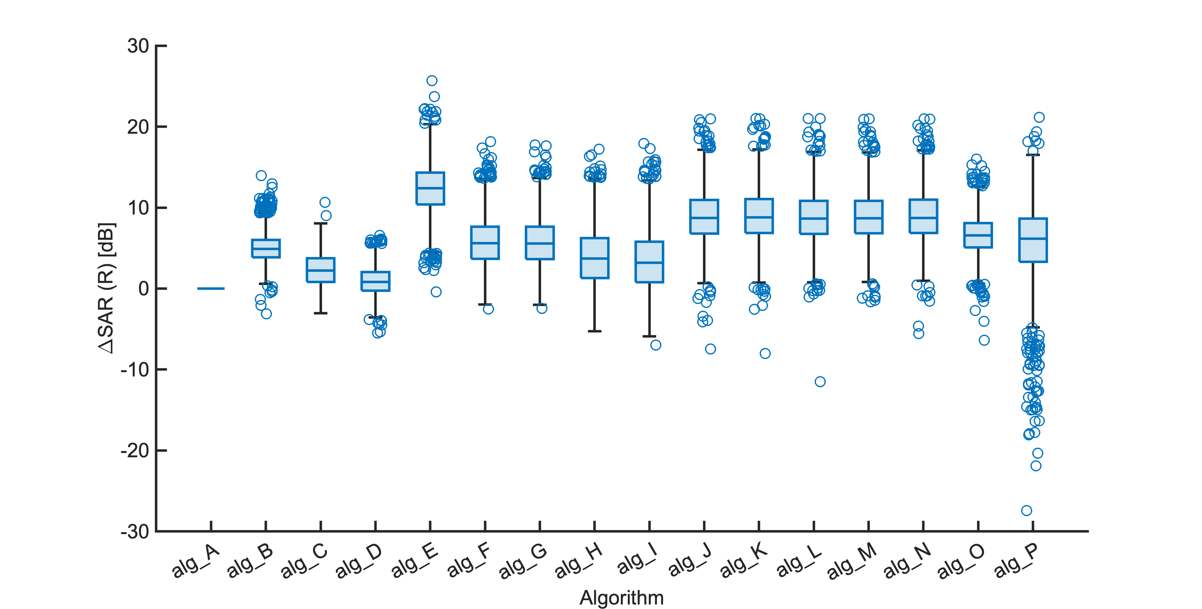
Each segment of enhanced audio was compared to the direct path in-ear signals using a large number of objective metrics (see Evaluation metrics). Here we show the difference in metric between each algorithm and the unprocessed noisy mixture (alg_A - passthrough).

Listening tests
Each pair of algorithms was compared by at least 10 participants. In each experiment 20 stimuli were presented.
Using a Bradley-Terry model as a hierarchical generalized model under a Bayesian framework to analyze the pair comparison data, the probability of the second algorithm in a specified ordered pair is dependent on the stimulus and the participant.
In the following figure, points represent median probability estimate of the 2nd algorithm being preferred; bars represent the 89% highest density credible interval surrounding the median estimate; asterisks indicate statistically significant probabilities (different from 0.5).

Considering all the pairwise data, the model predicts the number of times a particular algorithm would win in a fully balanced set of pairwise comparison trials. From this we obtain the rank order as shown below.
![]()