This practical introduces some simple techniques for visualising acoustic data in R by generating spectrograms from field recorder inputs. We can start by cleaning up your R environment and loading the required packages,
# Clear your global environment
rm(list = ls())

#load packages
library(tuneR)
library(seewave)
Now we need to get the path to a WAV file - we will use one of the Monkswood files. The data directory contains a set of files recorded across dawn on a single day.
#Check which sound files are in your directory
monkswood_files <- list.files(
    path='../data/Acoustics/Monkswood_dawn', pattern = "wav", full.names=TRUE
)
length(monkswood_files)head(monkswood_files)We can read in the first file and then look at some brief details on the kind of acoustic data in the file:
soundfile <- readWave(monkswood_files[1])

# Print the object to show details
print(soundfile)
Wave Object
	Number of Samples:      2880000
	Duration (seconds):     60
	Samplingrate (Hertz):   48000
	Channels (Mono/Stereo): Mono
	PCM (integer format):   TRUE
	Bit (8/16/24/32/64):    16
The recording contains a wider range of frequencies than we want to use, so we can apply
a simple band pass filter using the
seewave::fir() function to keep the the main bird calling frequencies.
# Filter out unwanted frequencies using 'fir()' function
soundfile <- fir(wave = soundfile,
                 from = 1000, # lower bound frequency in Hz
                 to = 20000, # upper bound frequency in Hz
                 bandpass = TRUE, output = "Wave")
We can then use the seewave::spectro() function to visualise the intensity of
different frequencies through time - a
spectrogram.
spectro(wave = soundfile, fastdisp=TRUE)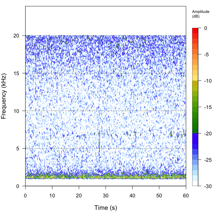
The seewave::spectro() function can be customised to show different parts of the WAV
file, filtering by frequency (flim) or time (tlim) limits. The plot below zooms in
on a 10 second section between 1 and 8 kHz:
spectro(wave = soundfile, fastdisp=TRUE,
        flim = c(1,8), # Set frequency limits of the spectrogram (kHz)
        tlim = c(10,20), #Set displayed time limits of the recording (sec)
        scale = TRUE, # Keeps the amplitude scale bar (FALSE to remove)
        colgrid = "gray", # Changes colour of the background grid
        palette = temp.colors, # Changes the colour palette
        dB="max0",
        cex.axis = 1.5, # Increase the axes label size
        cex.lab = 2) # Increase axes titles size)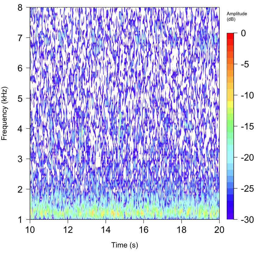
The next plot zooms in further to catch a specific call between 14 and 15 seconds into the recording:
spectro(wave = soundfile, fastdisp=TRUE,
        flim = c(1,8), # Set frequency limits of the spectrogram (kHz)
        tlim = c(14,15), #Set displayed time limits of the recording (sec)
        scale = TRUE, # Keeps the amplitude scale bar (FALSE to remove)
        colgrid = "gray", # Changes colour of the background grid
        palette = temp.colors, # Changes the colour palette
        dB="max0",
        cex.axis = 1.5, # Increase the axes label size
        cex.lab = 2) # Increase axes titles size)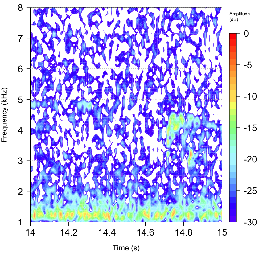
Finally, you can start a graphics device before creating the plot to export a spectrogram to file. The tricky part here is usually choosing an output file size in pixels that gives a good result.
# Start the graphics device
jpeg("outputs/Spectrogram_zoomed.jpg", width = 900, height = 500)

# Plot the spectrogram
spectro(wave = soundfile, flim = c(1,8),
        tlim = c(14,15),
        scale = TRUE,
        colgrid = "gray",
        palette = temp.colors,
        dB="max0",
        cex.axis = 1.5,
        cex.lab = 2
)
# Close the device to save the file
dev.off()The graphic below shows the exported JPEG file.
