Calculating Acoustic Indices in R - Ecological and Evolutionary Data Science

This practical introduces acoustic indices: values measured from an acoustic recording that have been designed to capture the acoustic environment along ecologically interesting axes. Again can start by cleaning up your R environment and loading the required packages.

# Clear your global environment
rm(list = ls())

#load packages
library(tuneR)
library(seewave)
library(stringr)
library(ggplot2)
library(patchwork)
library(soundecology)

Acoustic indices¶

We will use R to compare three acoustic indices. We will start by using the first file from Monkswood to compare the three indices:

audio <- readWave('../data/Acoustics/Monkswood_dawn/20240802_054502.wav')
print(audio)


Wave Object
	Number of Samples:      2880000
	Duration (seconds):     60
	Samplingrate (Hertz):   48000
	Channels (Mono/Stereo): Mono
	PCM (integer format):   TRUE
	Bit (8/16/24/32/64):    16

Acoustic Complexity Index¶

The acoustic complexity index is calculated using soundecology::acoustic_complexity(). See the function help for more details, but the basic idea is that biotic sounds tend to be more variable than human generated sounds.^[1]

# Calculate the ACI
aci_value <- acoustic_complexity(audio, min_freq = 1000, max_freq = 11000)


 This is a mono file.

 Calculating index. Please wait... 

  Acoustic Complexity Index (total): 757.7583

The return value is not just a single number - it is a complex object containing different parts of the calculation for the index - but the AciTotAll_left slot holds the actual ACI value:

str(aci_value)

List of 8
 $ AciTotAll_left       : num 758
 $ AciTotAll_right      : logi NA
 $ AciTotAll_left_bymin : num 758
 $ AciTotAll_right_bymin: logi NA
 $ aci_fl_left_vals     : num [1:107] 7.04 6.85 7.09 7.09 7.09 ...
 $ aci_fl_right_vals    : logi [1:12] NA NA NA NA NA NA ...
 $ aci_left_matrix      :'data.frame':	107 obs. of  12 variables:
  ..$ X1 : num [1:107] 0.578 0.575 0.594 0.572 0.599 ...
  ..$ X2 : num [1:107] 0.632 0.602 0.553 0.577 0.639 ...
  ..$ X3 : num [1:107] 0.587 0.578 0.604 0.601 0.61 ...
  ..$ X4 : num [1:107] 0.576 0.556 0.613 0.566 0.551 ...
  ..$ X5 : num [1:107] 0.562 0.58 0.575 0.591 0.595 ...
  ..$ X6 : num [1:107] 0.586 0.524 0.617 0.6 0.615 ...
  ..$ X7 : num [1:107] 0.605 0.562 0.616 0.564 0.547 ...
  ..$ X8 : num [1:107] 0.594 0.601 0.608 0.594 0.587 ...
  ..$ X9 : num [1:107] 0.573 0.585 0.571 0.602 0.556 ...
  ..$ X10: num [1:107] 0.59 0.597 0.54 0.591 0.607 ...
  ..$ X11: num [1:107] 0.576 0.569 0.602 0.601 0.574 ...
  ..$ X12: num [1:107] 0.586 0.517 0.599 0.629 0.606 ...
 $ aci_right_matrix     :'data.frame':	107 obs. of  12 variables:
  ..$ X1 : logi [1:107] NA NA NA NA NA NA ...
  ..$ X2 : logi [1:107] NA NA NA NA NA NA ...
  ..$ X3 : logi [1:107] NA NA NA NA NA NA ...
  ..$ X4 : logi [1:107] NA NA NA NA NA NA ...
  ..$ X5 : logi [1:107] NA NA NA NA NA NA ...
  ..$ X6 : logi [1:107] NA NA NA NA NA NA ...
  ..$ X7 : logi [1:107] NA NA NA NA NA NA ...
  ..$ X8 : logi [1:107] NA NA NA NA NA NA ...
  ..$ X9 : logi [1:107] NA NA NA NA NA NA ...
  ..$ X10: logi [1:107] NA NA NA NA NA NA ...
  ..$ X11: logi [1:107] NA NA NA NA NA NA ...
  ..$ X12: logi [1:107] NA NA NA NA NA NA ...

Normalized Difference Soundscape Index¶

Again, see the help on soundecology::ndsi() for details but the Normalized Difference Soundscape Index (NDSI) calculates an index as a ratio of indices of human-generated (anthrophony) to biological (biophony) acoustic.

# Calculate the NDSI
ndsi_value <- ndsi(audio)


 This is a mono file.

 Calculating index. Please wait... 

  Normalized Difference Soundscape Index: -0.3214462

Again, the return value is more complex than just a single number and includes the values of the separate biophony and anthrophony indices:

str(ndsi_value)

List of 6
 $ ndsi_left        : num -0.321
 $ ndsi_right       : logi NA
 $ biophony_left    : num 0.506
 $ anthrophony_left : num 0.985
 $ biophony_right   : logi NA
 $ anthrophony_right: logi NA

The NDSI value is then a normalised ratio of those two component.

round(
    (ndsi_value$biophony_left - ndsi_value$anthrophony_left) /
    (ndsi_value$biophony_left + ndsi_value$anthrophony_left),
3)

Bioacoustics Index¶

The bioacoustics index quantifies the amount of biophony in the signal: see soundecology::bioacoustic_index() for details.

# Calculate the BI
bi_value <- bioacoustic_index(audio, min_freq = 1000, max_freq = 11000)


 This is a mono file.

 Calculating index. Please wait... 

  Bioacoustic Index: 3.007625

This one actually does only return one value per channel:

str(bi_value)

List of 2
 $ left_area : num 3.01
 $ right_area: logi NA

Parallel processing¶

Loading all of the individual WAV files and processing each one in turn is:

Annoyingly complex, because you have to set up vectors to store results and then create a for loop to iterate over files and store results. ^[2]
Slow, because the files are processed one after the other (“in series”).

Fortunately, the soundecology::multiple_sounds function provides parallel processing of sound inputs in a directory and outputs the results to a CSV file. The three commands below run ACI, NDSI and BI for all files in the Monkswood dataset, using all the cores on your machine except for one (it is usually a good idea not to lock up all of your cores).

# Calculate acoustic_complexity using all but one core
multiple_sounds(
  directory = "../data/Acoustics/Monkswood_dawn",
  resultfile = "outputs/monkswood_aci.csv",
  soundindex = "acoustic_complexity",
  min_freq = 1000,
  max_freq = 11000,
  no_cores = -1
)


 Running the function acoustic_complexity() on 46 files using 9 cores

 The analysis of 46 files took 6.87 seconds

multiple_sounds(
  directory = "../data/Acoustics/Monkswood_dawn",
  resultfile = "outputs/monkswood_ndsi.csv",
  soundindex = "ndsi",
  no_cores = -1
)


 Running the function ndsi() on 46 files using 9 cores

 The analysis of 46 files took 14.85 seconds

multiple_sounds(
  directory = "../data/Acoustics/Monkswood_dawn",
  resultfile = "outputs/monkswood_bi.csv",
  soundindex = "bioacoustic_index",
  min_freq = 1000,
  max_freq = 11000,
  no_cores = -1
)


 Running the function bioacoustic_index() on 46 files using 9 cores

 The analysis of 46 files took 5.56 seconds

Assembling data¶

We now have three CSV files, one for each acoustic index, each of which contains a lot extra information that we do not need:

monkswood_bi <- read.csv("outputs/monkswood_bi.csv")
str(monkswood_bi)

'data.frame':	46 obs. of  11 variables:
 $ FILENAME     : chr  "20240802_054502.wav" "20240802_055002.wav" "20240802_055502.wav" "20240802_060002.wav" ...
 $ SAMPLINGRATE : int  48000 48000 48000 48000 48000 48000 48000 48000 48000 48000 ...
 $ BIT          : int  16 16 16 16 16 16 16 16 16 16 ...
 $ DURATION     : int  60 60 60 60 60 60 60 60 60 60 ...
 $ CHANNELS     : int  1 1 1 1 1 1 1 1 1 1 ...
 $ INDEX        : chr  "bioacoustic_index" "bioacoustic_index" "bioacoustic_index" "bioacoustic_index" ...
 $ FFT_W        : int  512 512 512 512 512 512 512 512 512 512 ...
 $ MIN_FREQ     : int  1000 1000 1000 1000 1000 1000 1000 1000 1000 1000 ...
 $ MAX_FREQ     : int  11000 11000 11000 11000 11000 11000 11000 11000 11000 11000 ...
 $ LEFT_CHANNEL : num  3.01 5.36 5.68 3.86 3.49 ...
 $ RIGHT_CHANNEL: chr  "NA " "NA " "NA " "NA " ...

monkswood_ndsi <- read.csv("outputs/monkswood_ndsi.csv")
str(monkswood_ndsi)

'data.frame':	46 obs. of  13 variables:
 $ FILENAME     : chr  "20240802_054502.wav" "20240802_055002.wav" "20240802_055502.wav" "20240802_060002.wav" ...
 $ SAMPLINGRATE : int  48000 48000 48000 48000 48000 48000 48000 48000 48000 48000 ...
 $ BIT          : int  16 16 16 16 16 16 16 16 16 16 ...
 $ DURATION     : int  60 60 60 60 60 60 60 60 60 60 ...
 $ CHANNELS     : int  1 1 1 1 1 1 1 1 1 1 ...
 $ INDEX        : chr  "ndsi" "ndsi" "ndsi" "ndsi" ...
 $ FFT_W        : int  1024 1024 1024 1024 1024 1024 1024 1024 1024 1024 ...
 $ ANTHRO_MIN   : int  1000 1000 1000 1000 1000 1000 1000 1000 1000 1000 ...
 $ ANTHRO_MAX   : int  2000 2000 2000 2000 2000 2000 2000 2000 2000 2000 ...
 $ BIO_MIN      : int  2000 2000 2000 2000 2000 2000 2000 2000 2000 2000 ...
 $ BIO_MAX      : int  11000 11000 11000 11000 11000 11000 11000 11000 11000 11000 ...
 $ LEFT_CHANNEL : num  -0.3214 -0.1301 0.0911 -0.5288 -0.4865 ...
 $ RIGHT_CHANNEL: chr  "NA " "NA " "NA " "NA " ...

monkswood_aci <- read.csv("outputs/monkswood_aci.csv")
str(monkswood_aci)

'data.frame':	46 obs. of  12 variables:
 $ FILENAME     : chr  "20240802_054502.wav" "20240802_055002.wav" "20240802_055502.wav" "20240802_060002.wav" ...
 $ SAMPLINGRATE : int  48000 48000 48000 48000 48000 48000 48000 48000 48000 48000 ...
 $ BIT          : int  16 16 16 16 16 16 16 16 16 16 ...
 $ DURATION     : int  60 60 60 60 60 60 60 60 60 60 ...
 $ CHANNELS     : int  1 1 1 1 1 1 1 1 1 1 ...
 $ INDEX        : chr  "acoustic_complexity" "acoustic_complexity" "acoustic_complexity" "acoustic_complexity" ...
 $ FFT_W        : int  512 512 512 512 512 512 512 512 512 512 ...
 $ MIN_FREQ     : int  1000 1000 1000 1000 1000 1000 1000 1000 1000 1000 ...
 $ MAX_FREQ     : int  11000 11000 11000 11000 11000 11000 11000 11000 11000 11000 ...
 $ J            : int  5 5 5 5 5 5 5 5 5 5 ...
 $ LEFT_CHANNEL : num  758 778 790 759 766 ...
 $ RIGHT_CHANNEL: chr  "NA " "NA " "NA " "NA " ...

The code below just simplifies these datarames to the information we want: it selects the file name and index value that is saved as LEFT_CHANNEL, and renames the fields with the index name.

monkswood_bi <- subset(monkswood_bi, select=c("FILENAME", "LEFT_CHANNEL"))
names(monkswood_bi) <- c("file", "bi")

monkswood_ndsi <- subset(monkswood_ndsi, select=c("FILENAME", "LEFT_CHANNEL"))
names(monkswood_ndsi) <- c("file", "ndsi")

monkswood_aci <- subset(monkswood_aci, select=c("FILENAME", "LEFT_CHANNEL"))
names(monkswood_aci) <- c("file", "aci")

We can now use merge to combine those files into a single dataframe: the function orders the inputs on the shared file field name and then combines the columns. We could use cbind to just join them together but that unsafely assumes that the results are written out in the same order.

monkswood_indices <- merge(merge(monkswood_bi,monkswood_ndsi), monkswood_aci)

Last, we can add a site label and then extract timestamps from the file name:

monkswood_indices$site <- "Monkswood"
monkswood_indices$datetime<-as.POSIXct(
  monkswood_indices$file, format = '%Y%m%d_%H%M%S.wav', tz = 'UTC'
)
monkswood_indices$date <- as.Date(monkswood_indices$datetime)
monkswood_indices$time <- format(monkswood_indices$datetime, format = "%H:%M")

head(monkswood_indices)

Visualising time series¶

The code below plots time series of each index using ggplot2 and the patchwork package for combining plots. We start by defining a theme - feel free to modify it to your own version!

theme_new <- function(base_size = 17, base_family = "Helvetica"){
  theme_classic(base_size = base_size, base_family = base_family) %+replace%
    theme(
      #line = element_line(colour="black"),
      #text = element_text(colour="black"),
      axis.text.x=element_text(colour = "black", size=17),
      axis.text.y=element_text(colour = "black", size=17),
      axis.title=element_text(size=21,face="bold"),
      legend.position = 'top', legend.direction = "horizontal",
      #strip.text = element_text(size=21),
      axis.line = element_line(colour = "black", linewidth = 1, linetype = "solid"),
      legend.key=element_rect(colour=NA, fill =NA),
      panel.grid = element_blank(),
      #panel.border = element_rect(fill = NA, colour = "black", size=0),
      #panel.background = element_rect(fill = "white", colour = "black"),
      #strip.background = element_rect(fill = NA)
    )
}

Next we can generate a plot object for each index. Here we use a useful ggplot2 trick that allows us to set a list of common ggplot2 elements we want to apply to each plot and recycle them. The resulting code is shorter and easier to update. The group = 1 syntax is required to tell ggplot that all the observations are in the same group and so the lines should be drawn between all points.

# Define shared ggplot elements
lineplot_elements <- list(
  geom_line(),
  scale_x_discrete(breaks=c("05:45","06:45","07:45", "08:45", "09:45")),
  labs(x = "Time"),
  theme_new()
)

ACI <- ggplot(monkswood_indices, aes(x=time, y=aci , group=1)) +
      labs(y = "ACI") +
      lineplot_elements

NDSI <- ggplot(monkswood_indices, aes(x=time, y=ndsi , group=1)) +
      labs(y = "NDSI") +
      lineplot_elements

BI <- ggplot(monkswood_indices, aes(x=time, y=bi , group=1)) +
      labs(y = "BI") +
      lineplot_elements

We can then use the / operator from patchwork to stack the plots and the plot_layout to remove the duplicated axes:

# Combine the three plots vertically
combined_plot <- ACI / BI / NDSI + plot_layout(axis_titles = "collect")
combined_plot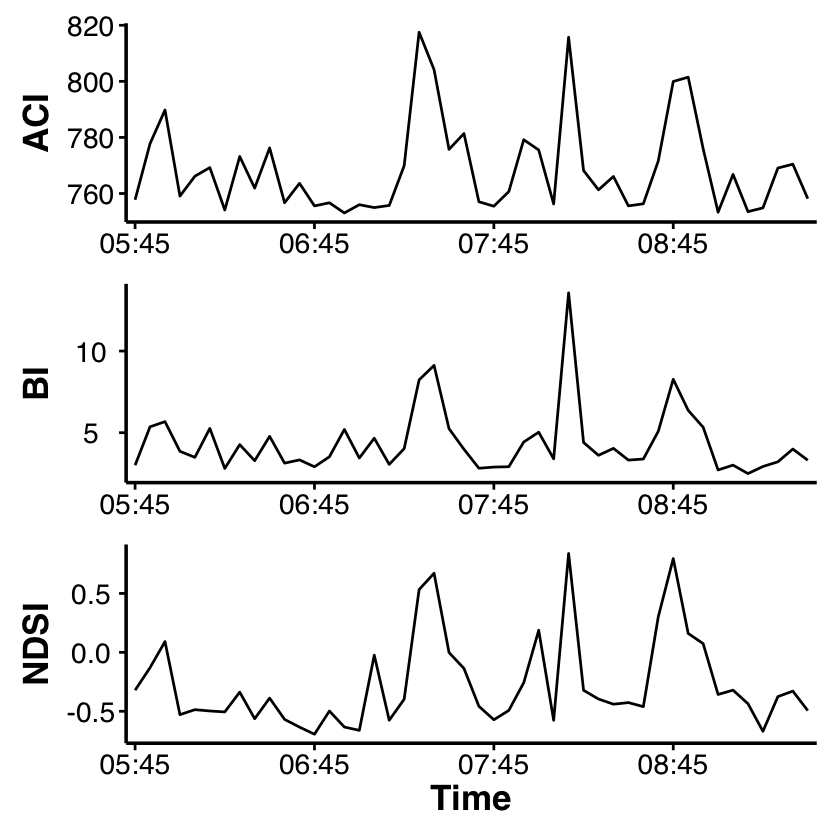

Comparing sites¶

The next steps are to compare the acoustic indices from Monkswood to the values for the Parsonage site.

Show solution

The code below runs the acoustic processing for the Parsonage data:

# Calculate indices
multiple_sounds(
  directory = "../data/Acoustics/Parsonage_dawn",
  resultfile = "outputs/parsonage_aci.csv",
  soundindex = "acoustic_complexity",
  min_freq = 1000,
  max_freq = 11000,
  no_cores = -1
)
multiple_sounds(
  directory = "../data/Acoustics/Parsonage_dawn",
  resultfile = "outputs/parsonage_ndsi.csv",
  soundindex = "ndsi",
  no_cores = -1
)
multiple_sounds(
  directory = "../data/Acoustics/Parsonage_dawn",
  resultfile = "outputs/parsonage_bi.csv",
  soundindex = "bioacoustic_index",
  min_freq = 1000,
  max_freq = 11000,
  no_cores = -1
)


 Running the function acoustic_complexity() on 46 files using 9 cores

 The analysis of 46 files took 5.96 seconds


 Running the function ndsi() on 46 files using 9 cores

 The analysis of 46 files took 13.37 seconds


 Running the function bioacoustic_index() on 46 files using 9 cores

 The analysis of 46 files took 5.42 seconds

Then the following code is used to combine the outputs into a single parsonage_indices dataframe with the same structure as the monkswood_indices dataframe

# Load and combine data
parsonage_bi <- read.csv("outputs/parsonage_bi.csv")
parsonage_ndsi <- read.csv("outputs/parsonage_ndsi.csv")
parsonage_aci <- read.csv("outputs/parsonage_aci.csv")

parsonage_bi <- subset(parsonage_bi, select=c("FILENAME", "LEFT_CHANNEL"))
names(parsonage_bi) <- c("file", "bi")
parsonage_ndsi <- subset(parsonage_ndsi, select=c("FILENAME", "LEFT_CHANNEL"))
names(parsonage_ndsi) <- c("file", "ndsi")
parsonage_aci <- subset(parsonage_aci, select=c("FILENAME", "LEFT_CHANNEL"))
names(parsonage_aci) <- c("file", "aci")
parsonage_indices <- merge(merge(parsonage_bi,parsonage_ndsi), parsonage_aci)

# Add extra data to dataframe
parsonage_indices$site <- "Parsonage"
parsonage_indices$datetime<-as.POSIXct(
  parsonage_indices$file, format = '%Y%m%d_%H%M%S.wav', tz = 'UTC'
)
parsonage_indices$date <- as.Date(parsonage_indices$datetime)
parsonage_indices$time <- format(parsonage_indices$datetime, format = "%H:%M")

Once you have created parsonage_indices, we can combine the sites into a single dataframe.

combined_indices <- rbind(monkswood_indices, parsonage_indices)

We can then generate plots comparing the two sites through the time series.

ACI <- ggplot(
    combined_indices,
    aes(x = time, y = aci, colour=site, group=site)
  ) +
  labs(y = "ACI") +
  lineplot_elements


NDSI <- ggplot(
    combined_indices,
    aes(x = time, y = ndsi, colour=site, group=site)
  ) +
  labs(y = "NDSI") +
  lineplot_elements

BI <- ggplot(
    combined_indices,
    aes(x = time, y = bi, colour=site, group=site)
  ) +
  labs(y = "BI")+
  lineplot_elements

# Vertically stack the plots, collect the legends and place them above the plot and
# collect the shared X axis labels.
combined_plot <- (ACI / BI / NDSI) +
  plot_layout(guides = "collect", axis_titles = "collect") &
  theme(legend.position = "top")

combined_plot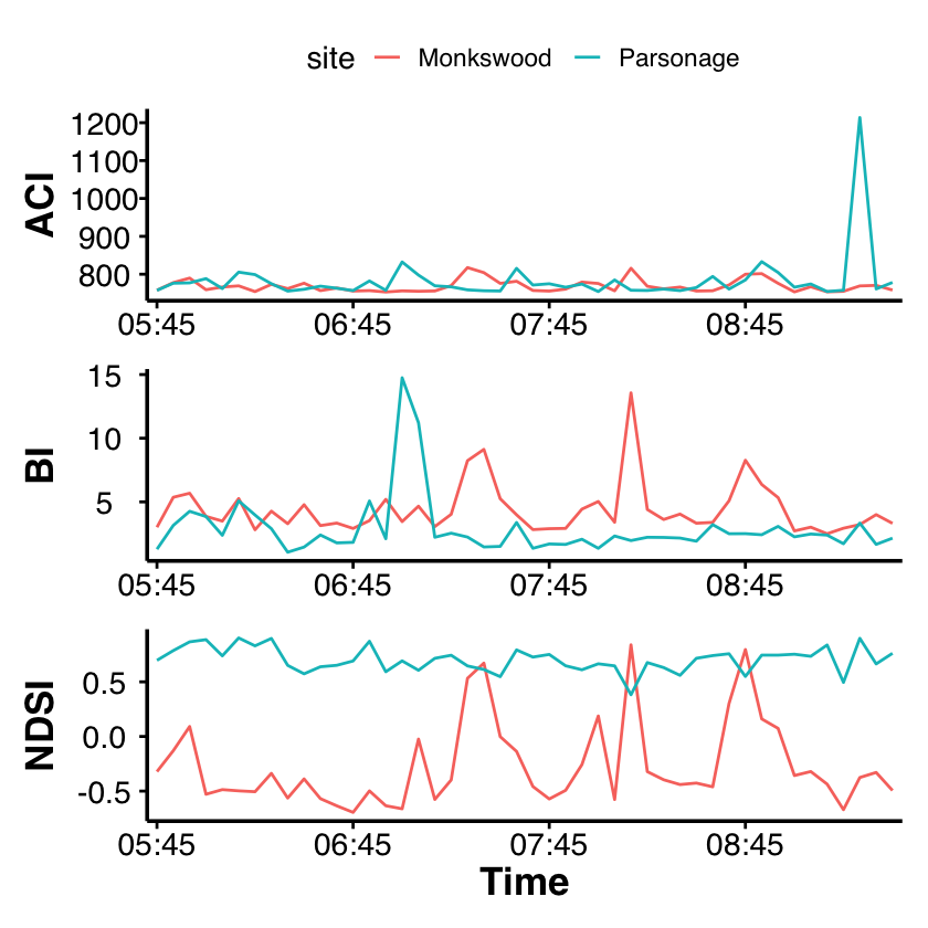

Statistical comparisons¶

It doesn’t look like there is any obvious temporal patterns in the acoustic indices above but the two sites do seem to have different average values. We can use boxplots to compare the average index values between sites:

# Shared boxplot ggplot2 elements
boxplot_elements <- list(
  geom_boxplot(),
  theme_new(),
  labs(title = "", x = "Site")
)


# Plots for ACI, BI, and NDSI
aci_boxplot <-   ggplot(
    data = combined_indices,
    aes(x = site, y = aci)
  ) +
  labs(y= "ACI Score") +
  boxplot_elements

bi_boxplot <-   ggplot(
    data = combined_indices,
    aes(x = site, y = bi)
  ) +
  labs(y= "BI Score") +
  boxplot_elements

ndsi_boxplot <-   ggplot(
    data = combined_indices,
    aes(x = site, y = ndsi)
  ) +
  labs(y= "NDSI Score") +
  boxplot_elements

# Combine the plots side by side
combined_boxplot <- (aci_boxplot + bi_boxplot + ndsi_boxplot)
combined_boxplot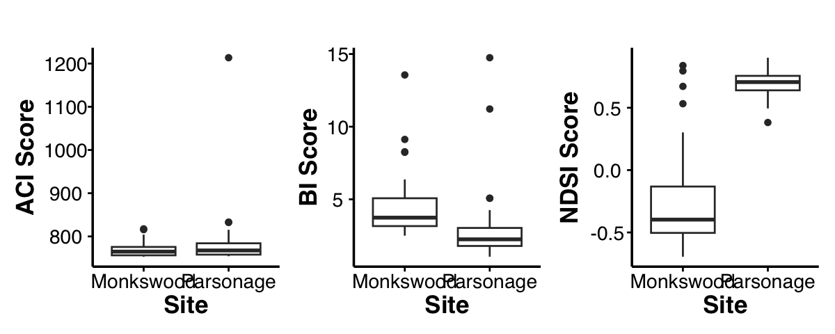

We can use statistical tests to see if there is a significant difference between sites. The code below uses a two sample Wilcoxon test. This is the non-parametric alternative to a T test for comparing continuous data from two categories and we are using it here because there are lots of outliers and fairly big differences in variance between the two sites.

wilcox.test(aci ~ site, data = combined_indices)


	Wilcoxon rank sum exact test

data:  aci by site
W = 855, p-value = 0.1141
alternative hypothesis: true location shift is not equal to 0

wilcox.test(bi ~ site, data = combined_indices)


	Wilcoxon rank sum exact test

data:  bi by site
W = 1807, p-value = 4.605e-10
alternative hypothesis: true location shift is not equal to 0

wilcox.test(ndsi ~ site, data = combined_indices)


	Wilcoxon rank sum exact test

data:  ndsi by site
W = 99, p-value < 2.2e-16
alternative hypothesis: true location shift is not equal to 0

Footnotes¶

The functions in the soundecology package print out quite a lot of processing information to the command line, and do not have a quiet option. The suppressMessages() function can be used to mute messages from noisy packages.
↩
You could load all the data into a list and use lapply, but WAV files are quite big so the memory usage does not scale well to large folders. The apply() family functions can also be hard to read and debug.
↩