Spatial methods in Ecological and Evolutionary Data Science - Ecological and Evolutionary Data Science

This webpage provides one long self-paced practical that provides an introduction to key spatial data handling and analysis techniques for use with the Ecological and Evolutionary Data Science. This practical uses the R programming language to load, manipulate and analyse spatial data. See more here on why we use R for GIS.

There are a lot of other sites that provide information on using R for GIS:

The core textbook for this practical is Geocomputation with R - it forms part of a broader set of resources from the geocompx group that provide resources for reproducible geographic data analysis, modeling, and visualization in several open source languages, also including Python and Julia.
Another great resource is the rspatial website, which provides a lot of information on using terra and other spatial tools in R.

Aims of the the practical¶

The practical aims to:

Provide you with some high quality spatial datasets for the Silwood and NHM sites that provide additional information that you can use to develop your hypotheses in your coursework for the module.
Run through most of the major GIS techniques that you will need to use to integrate raster and vector datasets in order to get to a final dataset addressing your hypotheses.
Provide simple plotting options using the basic R graphics commands. For more advanced mapping, see the “Making maps with R” chapter in “Geocomputation with R”.

How to use the practical¶

This practical is self-paced: work through it at your own speed and ask questions as needed! It builds up and then saves a set of datasets that you can use in your assessment, so you will need to:

Follow this guide on setting up packages and data for this practical.
Create a new R script file to run the practical analyses.
Copy example code from the practical into your script and run it from your script.
Check you understand what the code is doing - add extra comments, ask questions.
The practical contains exercises where you are asked to use the previous example to write and run your own code. Write your solution into your script file and again add comments for when you come back to it!
The practical contains solutions for all the exercises, but do try and solve them yourself.
At the end of the practical, you should have:
- A set of GIS data files that allow you to add further environmental context to the outputs of the sensor data exercises.
- A complete script that builds up those files from the original source data.

Required packages¶

We will need to load the following packages:

library(terra)       # core raster GIS package
library(sf)          # core vector GIS package
library(rcartocolor) # plotting
library(rpart)

You will see a whole load of package loading messages about GDAL, GEOS, PROJ which are not shown here. Don’t worry about this - they are not errors, just R linking to some key open source GIS toolkits.

Spatial datasets¶

We will be using a number of different datasets in both vector and raster format, at a range of resolutions. They are not all in the same projection and so we will need to supply coordinate system details. These can be very complex, but fortunately the EPSG database now provides a set of consistent codes that can be use to specify coordinate systems.

We will first load the location data from field datasets, which use GPS point location data in the WGS84 projection (EPSG:4326) with units in degrees:

The sensor deployment locations (16 sites across both the NHM and Silwood).
The blue tit nest box sites at Silwood (222 sites)

We will then load a set of additional data files in a wide range of formats. The following datasets are all downloaded from the Edina Digimap system. This is a UK national GIS resource for higher education, which you should be able to use for any UK based GIS whilst you are at the college using your college credentials. All of these datasets use the the OSGB36 / British National Grid projected coordinate system (EPSG:27700), with units in metres.

Aerial photography: RGB raster data at 25cm resolution with a single 3 x 3 km pane each of the two sites.
The Ordnance Survey (OS) Terrain 5 digital elevation dataset: raster data at 5m resolution with 2 pairs of 5 x 5 km panes for each site.
The CEH LandCover Map 2024: a raster land cover classification map with a single 3 x 3 km pane for each site.
The OS VectorMap Local dataset: two 5 x 5 km panes of vector data for each site.

There are then two final datasets:

Satellite data from the Sentinel 2 L2A product at a range of resolutions, using the Universal Transverse Mercator system. This projection uses multiple zones for different parts of the planet and the UK data is in UTM zone 30N (EPSG code EPSG:32630), with units of meters.
The GPS route for Silwood Christmas (Silmas) fun run and walking route. This is again in WGS84 projection.

The sections below show how to load each dataset.

Sensor locations¶

The sensor stations at Silwood and the NHM are recorded as a CSV file, providing station data including the latitude and longitude of each site. This file is directly downloaded from the Epicollect5 project. This is vector point data: precise locations from GPS associated with additional site data.

The data is first loaded as a simple CSV file.
We then need to convert the data to an sf (simple features) object. This is very like a normal R data frame, but contains an additional geometry field that contains the vector data geometries and the coordinate system. This is done using the sf::st_sf function to set the CSV fields that contain the point coordinates.

# Load the data from the CSV file
sensor_locations <- read.csv("../data/SensorSites/2025/sensor_sites_2025.csv")

# Convert to an sf object by setting the fields containing X and Y data and set 
# the projection of the dataset
sensor_locations <- st_as_sf(
  sensor_locations, 
  coords=c("long_Sensor_location","lat_Sensor_location"),
  crs="EPSG:4326"
)

Nest boxes¶

The locations of the Silwood blue tit nest boxes were also recorded using GPS. This is a long-term dataset and these data have already been processed into specific GIS format: the widely used shapefile format. The sf::st_read function is used to read existing GIS format files directly into an sf object.

nest_boxes <- st_read("../data/SpatialMethods/NestBoxes/NestBoxes.shp")

Reading layer `NestBoxes' from data source 
  `/Users/dorme/Teaching/GIS/living_planet_eco_evo_data/practicals/data/SpatialMethods/NestBoxes/NestBoxes.shp' 
  using driver `ESRI Shapefile'
replacing null geometries with empty geometries
Simple feature collection with 222 features and 9 fields (with 2 geometries empty)
Geometry type: POINT
Dimension:     XY
Bounding box:  xmin: -0.6544148 ymin: 51.40618 xmax: -0.638663 ymax: 51.41621
Geodetic CRS:  WGS 84

As you can see from the output above, loading a GIS file using sf::stread produces quite a lot of information. This practical handout will generally hide that to keep the page size down. We can also look at what an sf object looks like if you print it out: very like a dataframe with some extra header data.

print(head(nest_boxes))

Simple feature collection with 6 features and 9 fields
Geometry type: POINT
Dimension:     XY
Bounding box:  xmin: -0.6409471 ymin: 51.40993 xmax: -0.638663 ymax: 51.41213
Geodetic CRS:  WGS 84
  NestboxID TreeID TreeTag              Species Latitude  Longitude
1       A01   3938      NA fraxinus.excelsior¬† 51.40993 -0.6386630
2       A03    611    1322        quercus.robur 51.41107 -0.6400258
3       A04   3847      NA  acer.pseudoplatanus 51.41167 -0.6393205
4       A05   3859      NA       betula.pendula 51.41195 -0.6403336
5       A06    636    1351        quercus.robur 51.41196 -0.6407162
6       A07    660    5772        quercus.robur 51.41213 -0.6409471
         SPlocation Type State                    geometry
1 Observatory copse   26 alive  POINT (-0.638663 51.40993)
2 Observatory copse   26 alive POINT (-0.6400258 51.41107)
3 Observatory copse   26 alive POINT (-0.6393205 51.41167)
4 Observatory copse   26 alive POINT (-0.6403336 51.41195)
5    Merten's acres   26 alive POINT (-0.6407162 51.41196)
6    Merten's acres   26 alive POINT (-0.6409471 51.41213)

Woodland survey¶

The Silwood woodland survey transect points: another CSV file providing latitude and longitude of transect locations.

TODO

Aerial photography¶

These raster datasets provide 3km by 3km panes of 25cm resolution aerial photography imagery for the two sites. These files are provided as GeoTIFF data files - these are essentially just standard TIFF image files but contain metadata that provides the spatial context of each pixel in the image and the projection information.

Raster data can be loaded using the terra::rast function.

nhm_aerial <- rast('../data/SpatialMethods/aerial/nhm_aerial.tiff')
silwood_aerial <- rast('../data/SpatialMethods/aerial/silwood_aerial.tiff')

Printing out one of those fhiles shows the spatial information of the raster and then a table showing the names of the bands in the raster and their range. These files contain three band to provide RGB imagery.

print(nhm_aerial)

class       : SpatRaster 
size        : 12000, 12000, 3  (nrow, ncol, nlyr)
resolution  : 0.25, 0.25  (x, y)
extent      : 525000, 528000, 178000, 181000  (xmin, xmax, ymin, ymax)
coord. ref. : OSGB36 / British National Grid (EPSG:27700) 
source      : nhm_aerial.tiff 
names       : tq2578_rgb_250_09_1, tq2578_rgb_250_09_2, tq2578_rgb_250_09_3 
min values  :                   0,                   6,                   5 
max values  :                 255,                 255,                 255

OS Terrain 5¶

These raster datasets provide continuous elevation data at 5m resolution from the Ordnance Survey Terrain 5 Digital Terrain Map (DTM) dataset. Each site has two adjoining panes of data.

These files are ASC format files - a very simple text based format that contains the cell coordinates but not the projection metadata, so we need to add that information.

# Load the DTM data from ASC format files
silwood_dtm_SU96NE <- rast("../data/SpatialMethods/dtm_5m/SU96NE.asc")
silwood_dtm_SU96NW <- rast("../data/SpatialMethods/dtm_5m/SU96NW.asc")
nhm_dtm_TQ27NE <- rast("../data/SpatialMethods/dtm_5m/TQ27NE.asc")
nhm_dtm_TQ28SE <- rast("../data/SpatialMethods/dtm_5m/TQ28SE.asc")

If we look at one of those datasets, you can see that the cell coordinates, resolution and overall dataset size have been set but that the coord. ref attribute is empty.

# Look at the object data
silwood_dtm_SU96NE

class       : SpatRaster 
size        : 1000, 1000, 1  (nrow, ncol, nlyr)
resolution  : 5, 5  (x, y)
extent      : 495000, 5e+05, 165000, 170000  (xmin, xmax, ymin, ymax)
coord. ref. :  
source      : SU96NE.asc 
name        : SU96NE

We need to set the projection manually using the terra::crs function and then check that the attribute has been set.

# Set the projection information for the DTM datasets
crs(silwood_dtm_SU96NE) <- crs(silwood_dtm_SU96NW) <- "EPSG:27700"
crs(nhm_dtm_TQ27NE) <- crs(nhm_dtm_TQ28SE) <- "EPSG:27700"

# Print the modified dataset
silwood_dtm_SU96NE

class       : SpatRaster 
size        : 1000, 1000, 1  (nrow, ncol, nlyr)
resolution  : 5, 5  (x, y)
extent      : 495000, 5e+05, 165000, 170000  (xmin, xmax, ymin, ymax)
coord. ref. : OSGB36 / British National Grid (EPSG:27700) 
source      : SU96NE.asc 
name        : SU96NE

CEH Land Cover¶

The Centre for Ecology and Hydrology produces a UK wide land cover map at 10 metre resolution. The datasets here are taken from the most recent Land Cover Map 2024.

The land cover categories are assigned using a classification of multi-band spectral data from satellites onto the spectral signatures of known training sites. Each cell is assigned to the category with training signatures that most closely match the spectral signature of the cell.

# Load the land cover map datasets
silwood_LCM <- rast("../data/SpatialMethods/lcm_2024/Silwood_LCM2024.tiff")
nhm_LCM <- rast("../data/SpatialMethods/lcm_2024/NHM_LCM2024.tiff")

# Look at the raster details
print(silwood_LCM)

class       : SpatRaster 
size        : 300, 300, 2  (nrow, ncol, nlyr)
resolution  : 10, 10  (x, y)
extent      : 493000, 496000, 167000, 170000  (xmin, xmax, ymin, ymax)
coord. ref. : OSGB36 / British National Grid (EPSG:27700) 
source      : Silwood_LCM2024.tiff 
names       : gblcm2024_10m_1, gblcm2024_10m_2 
min values  :               1,              13 
max values  :              21,             100

The LCM2024 files contain two raster bands. The first band is a numeric code giving the land cover category. The second band give the probability of the cell having that land cover type, based on the underlying classification. As loaded, these values are just numeric, so if we plot the data, we will get two continuous colour legends:

plot(silwood_LCM)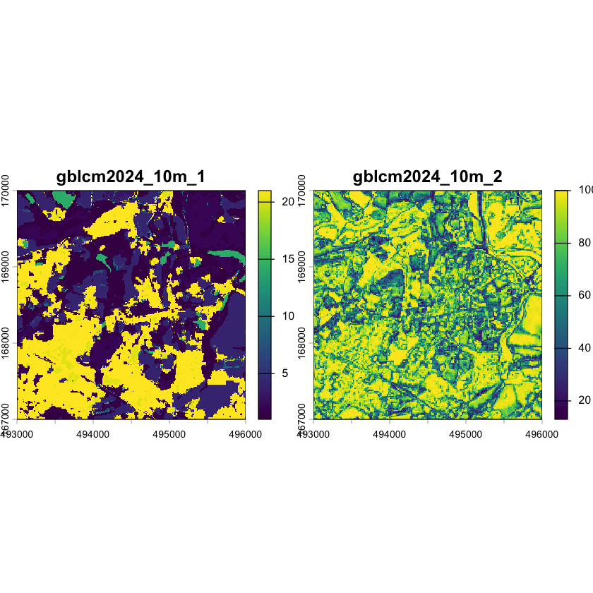

We can add category labels and better category colours to make the data easier to use. The labels and some colours are defined in a separate CSV file:

lcm_info <- read.csv("../data/SpatialMethods/lcm_2024/LCM2024_info.csv")

# Set the band names, the category code labels and the colour tables
levels(nhm_LCM) <- lcm_info[c("value", "label")]
coltab(nhm_LCM) <- lcm_info[c("value", "color")]
names(nhm_LCM) <- c("LandCover", "Certainty")

coltab(silwood_LCM) <- lcm_info[c("value", "color")]
levels(silwood_LCM) <- lcm_info[c("value", "label")]
names(silwood_LCM) <- c("LandCover", "Certainty")

Now we can now plot maps that have actual category labels:

par(mfrow=c(1,2))
plot(silwood_LCM["LandCover"])
plot(nhm_LCM["LandCover"])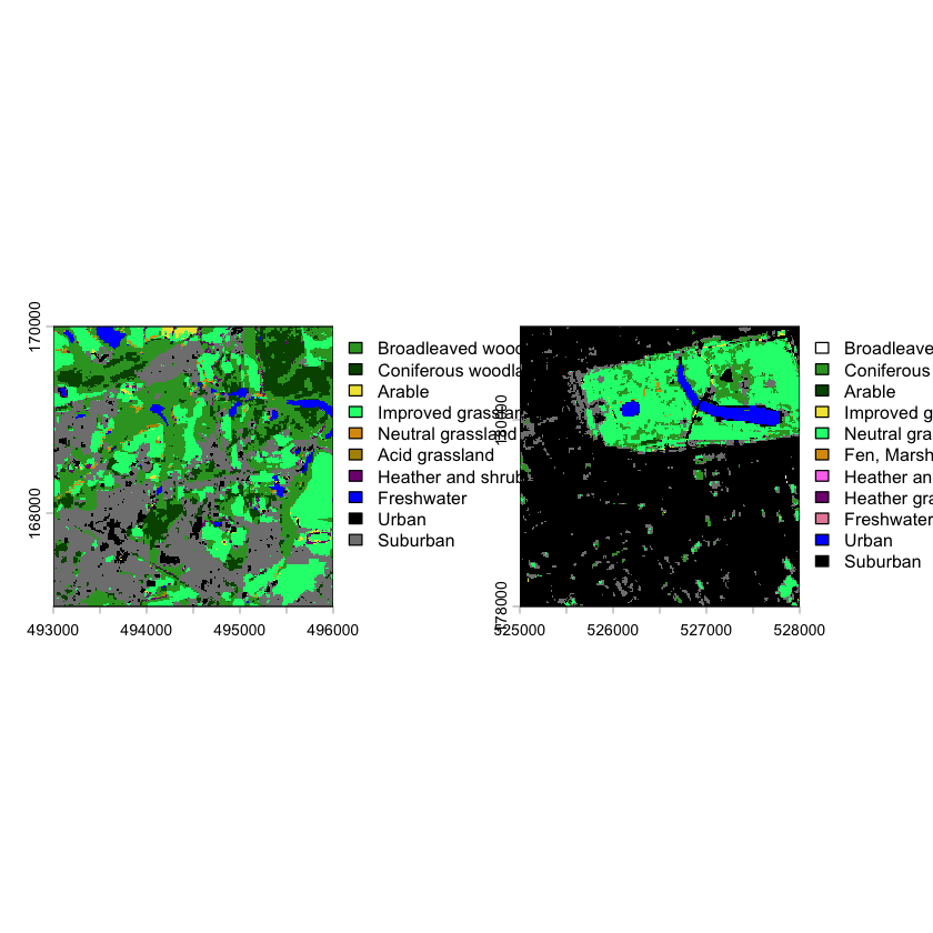

And look at the frequencies of the different categories using the terra::freq function:

nhm_freq <- freq(nhm_LCM["LandCover"])
silwood_freq <- freq(silwood_LCM["LandCover"])

# Join the two datasets, including all categories
merge(
  nhm_freq, silwood_freq, 
  by="value", all=TRUE, suffixes = c(".nhm", ".silwood")
)

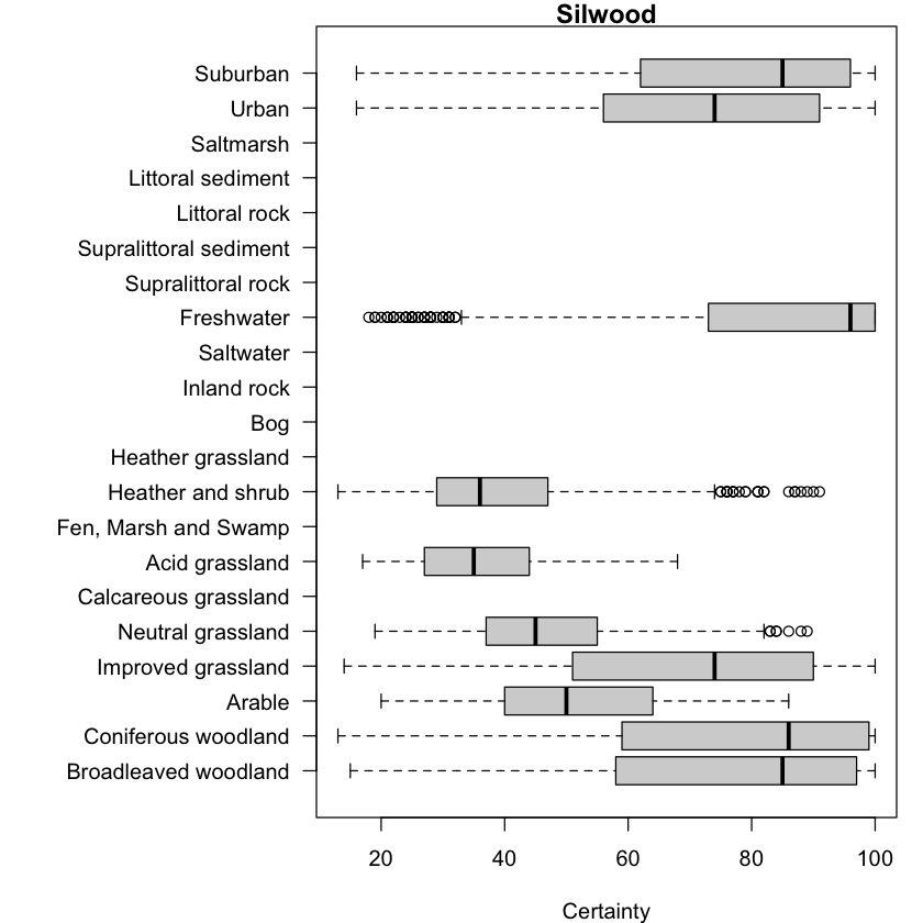
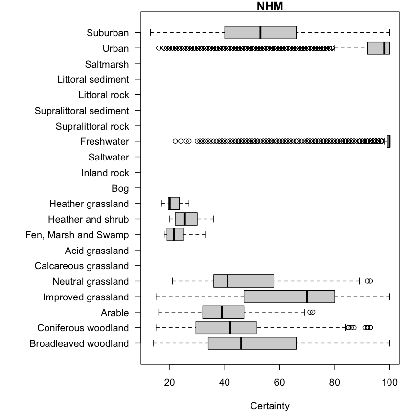
We can also use the data within raster layers with other non-spatial data exploration techniques. For example, we can look at the distribution of cell certainties associated with each category.

par(mar = c(4, 12, 1, 1))

# Plot cell assignment certainties as a function of land cover category
boxplot(
  silwood_LCM["Certainty"], silwood_LCM["LandCover"], 
  las = 1, ylab = "", horizontal=TRUE, main="Silwood", xlab="Certainty"
)
boxplot(
  nhm_LCM["Certainty"], nhm_LCM["LandCover"], 
  las = 1, ylab = "", horizontal=TRUE, main="NHM", xlab="Certainty"
)

OS VectorMap Local¶

The Ordnance Survey VectorMap Local dataset provides very high precision vector data on spatial features in the UK. These files are saved in the GeoPackage file format (.gpkg). As with the Terrain 5 data, the data from Edina Digimap consists of two 5 x 5 km panes for each site.

A GeoPackage file can contain multiple vector datasets in a single file: these are usually called “layers” and so you will typically load one layer at a time. The code below uses the sf::st_layers command to show the available layers within one of the VML datasets.

print(st_layers("../data/SpatialMethods/VML/vml-su96ne.gpkg"))

Driver: GPKG 
Available layers:
                layer_name geometry_type features fields
1            Landform_Area       Polygon     1137      3
2             Urban_Extent       Polygon        5      3
3                 Building       Polygon     3776      3
4               Water_Area       Polygon      197      3
5                   Bridge       Polygon        1      3
6             General_Line   Line String    17433      3
7            Building_Line   Line String     3839      3
8          Height_Contours   Line String      251      3
9            Landform_Line   Line String      101      3
10              Water_Line   Line String      659      3
11 Administrative_Boundary   Line String       11      3
12         Rail_Centreline   Line String       41      3
13         Road_Centreline   Line String     1333      5
14            General_Text         Point      366      9
15    Road_Centreline_Text         Point     1564      9
16           Building_Text         Point      120      9
17             Height_Text         Point      247      9
18              Water_Text         Point       97      9
19           General_Point         Point       20      5
20            Water_Points         Point       69      5
21           Height_Points         Point       93      5
                         crs_name
1  OSGB36 / British National Grid
2  OSGB36 / British National Grid
3  OSGB36 / British National Grid
4  OSGB36 / British National Grid
5  OSGB36 / British National Grid
6  OSGB36 / British National Grid
7  OSGB36 / British National Grid
8  OSGB36 / British National Grid
9  OSGB36 / British National Grid
10 OSGB36 / British National Grid
11 OSGB36 / British National Grid
12 OSGB36 / British National Grid
13 OSGB36 / British National Grid
14 OSGB36 / British National Grid
15 OSGB36 / British National Grid
16 OSGB36 / British National Grid
17 OSGB36 / British National Grid
18 OSGB36 / British National Grid
19 OSGB36 / British National Grid
20 OSGB36 / British National Grid
21 OSGB36 / British National Grid

We can then use the sf::st_read function to read specific different layers for each site.

# Load the two panes of VML road centrelines for each site.
vml_tq28se_roads <- st_read(
  dsn = "../data/SpatialMethods/VML/vml-tq28se.gpkg", layer = "Road_Centreline"
)
vml_tq27ne_roads <- st_read(
  dsn = "../data/SpatialMethods/VML/vml-tq27ne.gpkg", layer = "Road_Centreline"
)
vml_su96ne_roads <- st_read(
  dsn = "../data/SpatialMethods/VML/vml-su96ne.gpkg", layer = "Road_Centreline"
)
vml_su96nw_roads <- st_read(
  dsn = "../data/SpatialMethods/VML/vml-su96nw.gpkg", layer = "Road_Centreline"
)

# Do the same for water bodies
vml_tq28se_water <- st_read(
  dsn = "../data/SpatialMethods/VML/vml-tq28se.gpkg", layer = "Water_Area"
)
vml_tq27ne_water <- st_read(
  dsn = "../data/SpatialMethods/VML/vml-tq27ne.gpkg", layer = "Water_Area"
)
vml_su96ne_water <- st_read(
  dsn = "../data/SpatialMethods/VML/vml-su96ne.gpkg", layer = "Water_Area"
)
vml_su96nw_water <- st_read(
  dsn = "../data/SpatialMethods/VML/vml-su96nw.gpkg", layer = "Water_Area"
)

Reading layer `Road_Centreline' from data source 
  `/Users/dorme/Teaching/GIS/living_planet_eco_evo_data/practicals/data/SpatialMethods/VML/vml-tq28se.gpkg' 
  using driver `GPKG'
Simple feature collection with 8916 features and 5 fields
Geometry type: LINESTRING
Dimension:     XY
Bounding box:  xmin: 524731 ymin: 179744.5 xmax: 530112 ymax: 185228.1
Projected CRS: OSGB36 / British National Grid

Reading layer `Road_Centreline' from data source 
  `/Users/dorme/Teaching/GIS/living_planet_eco_evo_data/practicals/data/SpatialMethods/VML/vml-tq27ne.gpkg' 
  using driver `GPKG'
Simple feature collection with 8122 features and 5 fields
Geometry type: LINESTRING
Dimension:     XY
Bounding box:  xmin: 524579.6 ymin: 174853.7 xmax: 530153.2 ymax: 180470.7
Projected CRS: OSGB36 / British National Grid

Reading layer `Road_Centreline' from data source 
  `/Users/dorme/Teaching/GIS/living_planet_eco_evo_data/practicals/data/SpatialMethods/VML/vml-su96ne.gpkg' 
  using driver `GPKG'
Simple feature collection with 1333 features and 5 fields
Geometry type: LINESTRING
Dimension:     XY
Bounding box:  xmin: 494774.3 ymin: 164397 xmax: 500586 ymax: 170268.6
Projected CRS: OSGB36 / British National Grid

Reading layer `Road_Centreline' from data source 
  `/Users/dorme/Teaching/GIS/living_planet_eco_evo_data/practicals/data/SpatialMethods/VML/vml-su96nw.gpkg' 
  using driver `GPKG'
Simple feature collection with 1956 features and 5 fields
Geometry type: LINESTRING
Dimension:     XY
Bounding box:  xmin: 488519.8 ymin: 164588.5 xmax: 495366 ymax: 170367.4
Projected CRS: OSGB36 / British National Grid

Reading layer `Water_Area' from data source 
  `/Users/dorme/Teaching/GIS/living_planet_eco_evo_data/practicals/data/SpatialMethods/VML/vml-tq28se.gpkg' 
  using driver `GPKG'
Simple feature collection with 129 features and 3 fields
Geometry type: POLYGON
Dimension:     XY
Bounding box:  xmin: 524874.3 ymin: 179936 xmax: 530118.6 ymax: 184188.5
Projected CRS: OSGB36 / British National Grid

Reading layer `Water_Area' from data source 
  `/Users/dorme/Teaching/GIS/living_planet_eco_evo_data/practicals/data/SpatialMethods/VML/vml-tq27ne.gpkg' 
  using driver `GPKG'
Simple feature collection with 113 features and 3 fields
Geometry type: POLYGON
Dimension:     XY
Bounding box:  xmin: 525000 ymin: 174967.8 xmax: 530019.1 ymax: 180203.8
Projected CRS: OSGB36 / British National Grid

Reading layer `Water_Area' from data source 
  `/Users/dorme/Teaching/GIS/living_planet_eco_evo_data/practicals/data/SpatialMethods/VML/vml-su96ne.gpkg' 
  using driver `GPKG'
Simple feature collection with 197 features and 3 fields
Geometry type: POLYGON
Dimension:     XY
Bounding box:  xmin: 494889.5 ymin: 164949.9 xmax: 500058.7 ymax: 170239.3
Projected CRS: OSGB36 / British National Grid

Reading layer `Water_Area' from data source 
  `/Users/dorme/Teaching/GIS/living_planet_eco_evo_data/practicals/data/SpatialMethods/VML/vml-su96nw.gpkg' 
  using driver `GPKG'
Simple feature collection with 241 features and 3 fields
Geometry type: POLYGON
Dimension:     XY
Bounding box:  xmin: 489969.7 ymin: 165112.2 xmax: 495114.6 ymax: 170260.6
Projected CRS: OSGB36 / British National Grid

Sentinel 2 data¶

The Sentinel 2 satellite mission collects spectral data from 13 bands across the visible, near infra-red and infra-red at resolutions from 10m to 60m. See the Copernicus Sentinel 2 data wiki for more information about the mission and data processing.

The sentinel_2 folder contains data from a single (relatively cloud free!) scene from the Sentinel 2 Level 2A data product that was downloaded using the Copernicus data browser. The L2A data product has been processed to remove atmospheric effects to give modelled surface reflectance values for each band and also to add some extra calculated layers, such as true colour images (more on this later!).

A single scene of L2A data covers roughly 110 x 110 km and contains about 1 GB of data, so has been cropped down to the two study sites (see below). The code below loads the four 10m resolution bands into a single raster for each site by providing a vector of file names to the terra::rast function. It also rescales the data: remote sensing data is often stored as integer data to save file space and needs converting to actual values, in this case by dividing by 10000.

# Load the four 10m resolution Sentinel 2 bands for Silwood
s2_silwood_10m <- rast(
    c(
        "../data/SpatialMethods/sentinel_2/R10m/silwood/T30UXC_20250711T110651_B02_10m.tiff",
        "../data/SpatialMethods/sentinel_2/R10m/silwood/T30UXC_20250711T110651_B03_10m.tiff",
        "../data/SpatialMethods/sentinel_2/R10m/silwood/T30UXC_20250711T110651_B04_10m.tiff",
        "../data/SpatialMethods/sentinel_2/R10m/silwood/T30UXC_20250711T110651_B08_10m.tiff"
    ),
)  / 10000

# Name the bands 
names(s2_silwood_10m) <- c("B", "G", "R", "NIR")

# Do the same for the NHM
s2_nhm_10m <- rast(
    c(
        "../data/SpatialMethods/sentinel_2/R10m/nhm/T30UXC_20250711T110651_B02_10m.tiff",
        "../data/SpatialMethods/sentinel_2/R10m/nhm/T30UXC_20250711T110651_B03_10m.tiff",
        "../data/SpatialMethods/sentinel_2/R10m/nhm/T30UXC_20250711T110651_B04_10m.tiff",
        "../data/SpatialMethods/sentinel_2/R10m/nhm/T30UXC_20250711T110651_B08_10m.tiff"
    ),
) / 10000
names(s2_nhm_10m) <- c("B", "G", "R", "NIR")

# Show the resulting object structure
print(s2_silwood_10m)

class       : SpatRaster 
size        : 312, 312, 4  (nrow, ncol, nlyr)
resolution  : 10, 10  (x, y)
extent      : 662390, 665510, 5696240, 5699360  (xmin, xmax, ymin, ymax)
coord. ref. : WGS 84 / UTM zone 30N (EPSG:32630) 
source(s)   : memory
names       :      B,     G,      R,    NIR 
min values  : 0.1067, 0.110, 0.1085, 0.1060 
max values  : 0.5808, 0.616, 0.6088, 0.7964

Show solution

# Load the six 20m resolution Sentinel 2 bands for Silwood
s2_silwood_20m <- rast(
    c(
        "../data/SpatialMethods/sentinel_2/R20m/silwood/T30UXC_20250711T110651_B05_20m.tiff",
        "../data/SpatialMethods/sentinel_2/R20m/silwood/T30UXC_20250711T110651_B06_20m.tiff",
        "../data/SpatialMethods/sentinel_2/R20m/silwood/T30UXC_20250711T110651_B07_20m.tiff",
        "../data/SpatialMethods/sentinel_2/R20m/silwood/T30UXC_20250711T110651_B8A_20m.tiff",
        "../data/SpatialMethods/sentinel_2/R20m/silwood/T30UXC_20250711T110651_B11_20m.tiff",
        "../data/SpatialMethods/sentinel_2/R20m/silwood/T30UXC_20250711T110651_B12_20m.tiff"
    ),
) / 10000

# Name the bands 
names(s2_silwood_20m) <- c("RE5", "RE6", "RE7", "NNIR", "SWIR1", "SWIR2")

# Load the seven 20m resolution Sentinel 2 bands for the NHM
s2_nhm_20m <- rast(
    c(
        "../data/SpatialMethods/sentinel_2/R20m/nhm/T30UXC_20250711T110651_B05_20m.tiff",
        "../data/SpatialMethods/sentinel_2/R20m/nhm/T30UXC_20250711T110651_B06_20m.tiff",
        "../data/SpatialMethods/sentinel_2/R20m/nhm/T30UXC_20250711T110651_B07_20m.tiff",
        "../data/SpatialMethods/sentinel_2/R20m/nhm/T30UXC_20250711T110651_B8A_20m.tiff",
        "../data/SpatialMethods/sentinel_2/R20m/nhm/T30UXC_20250711T110651_B11_20m.tiff",
        "../data/SpatialMethods/sentinel_2/R20m/nhm/T30UXC_20250711T110651_B12_20m.tiff"
    ),
) / 10000

# Name the bands 
names(s2_nhm_20m) <- c("RE5", "RE6", "RE7", "NNIR", "SWIR1", "SWIR2")

Silmas walk/run route¶

The last dataset is a GPS Exchange Format (GPX) file containing the course of the Silmas fun run and walking route. The GPX format is a commonly used format to record routes and points from GPS devices. Again, the format holds multiple layers:

print(st_layers("../data/SpatialMethods/Silmas_Fun_Run.gpx"))

Driver: GPX 
Available layers:
    layer_name     geometry_type features fields crs_name
1    waypoints             Point        0     23   WGS 84
2       routes       Line String        0     12   WGS 84
3       tracks Multi Line String        1     12   WGS 84
4 route_points             Point        0     25   WGS 84
5 track_points             Point      425     26   WGS 84

With GPX files, there are a fixed number of layers. They are not all used in this file: we have a single linear feature in tracks layer, which is the Silmas route, and then the 425 point features in the track_points layer, which are the points along along that route. We will load the tracks layer:

silmas_route <- st_read(
  dsn="../data/SpatialMethods/Silmas_Fun_Run.gpx", layer="tracks"
)

Reading layer `tracks' from data source 
  `/Users/dorme/Teaching/GIS/living_planet_eco_evo_data/practicals/data/SpatialMethods/Silmas_Fun_Run.gpx' 
  using driver `GPX'
Simple feature collection with 1 feature and 12 fields
Geometry type: MULTILINESTRING
Dimension:     XY
Bounding box:  xmin: -0.650703 ymin: 51.40805 xmax: -0.63996 ymax: 51.42044
Geodetic CRS:  WGS 84

Plotting GIS data¶

Plotting vector data¶

If you plot a vector dataset, then it will generate a panel for each vector attribute in the dataset (up to a limit!).

plot(nest_boxes)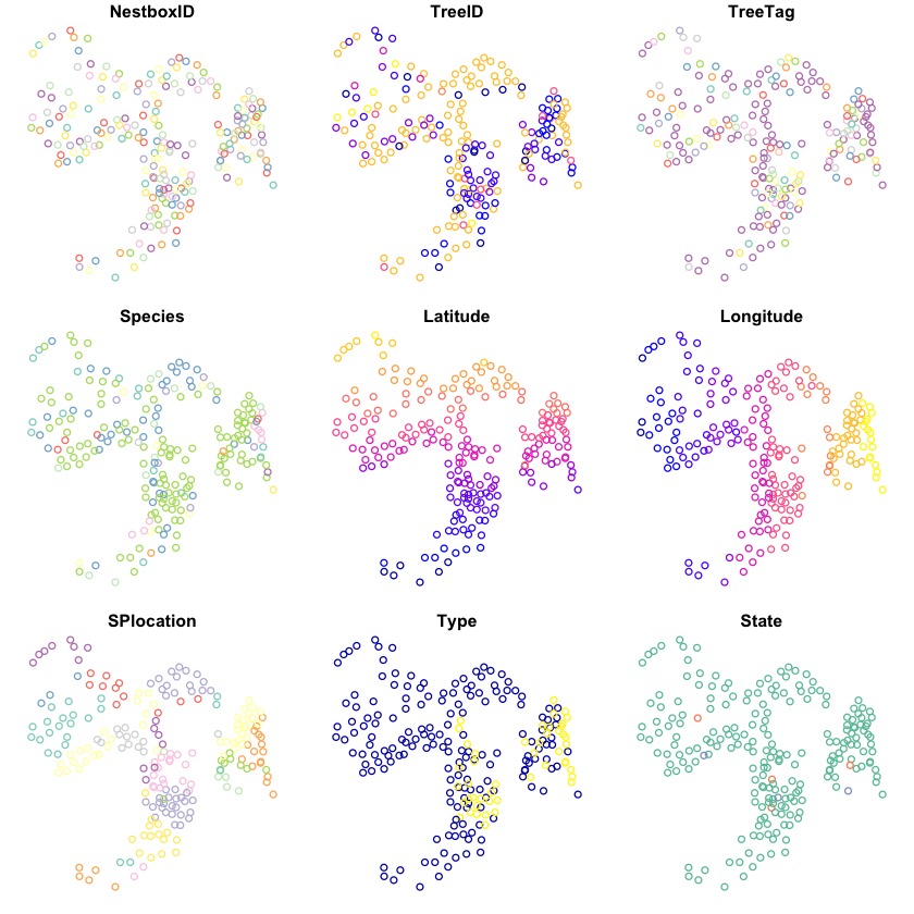

If you want to plot just one of those attributes, then you can use [] subsets to do so, and R will generate a key for it.

plot(nest_boxes['SPlocation'], key.pos=4)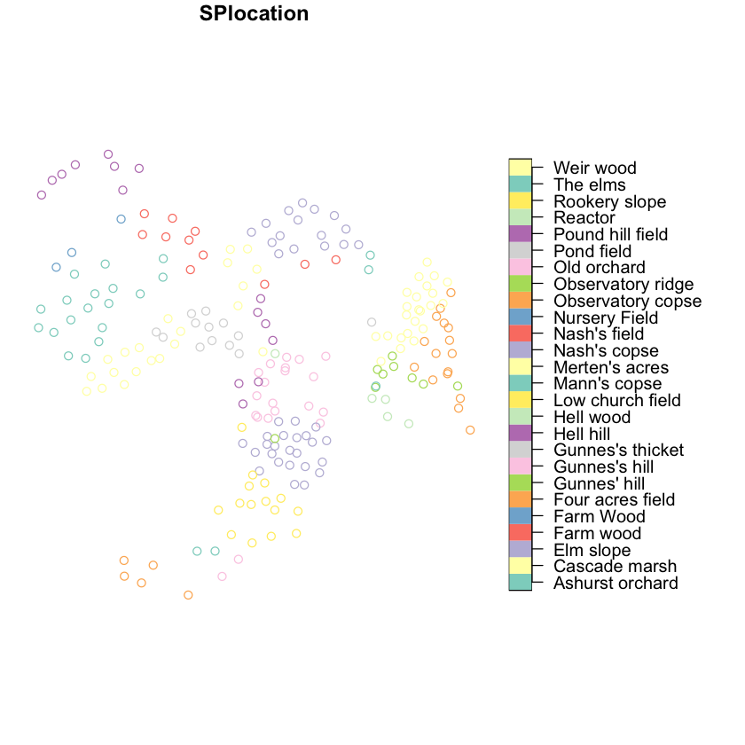

If you just want to plot the features geometry, then you can use sf::st_geometry. You can use add=TRUE to overplot features and you can use extent to change the spatial area being plotted. It can be tricky to set the area of the plot so that it will include all features. One trick here is to get the extent (or bounding box) of the layers you want to plot and then convert them to polygons using sf::st_as_sfc and then take the spatial union(sf::st_union) of those boxes. Long-winded but reliable!

# Get the plot extent as the union of the bounding boxes
plot_extent <- st_union(
  st_as_sfc(st_bbox(nest_boxes)),
  st_as_sfc(st_bbox(silmas_route))
)

# Plot the nest box points and overplot the Silmas route
plot(st_geometry(nest_boxes), col="forestgreen", extent=plot_extent)
plot(st_geometry(silmas_route), col="red", add=TRUE)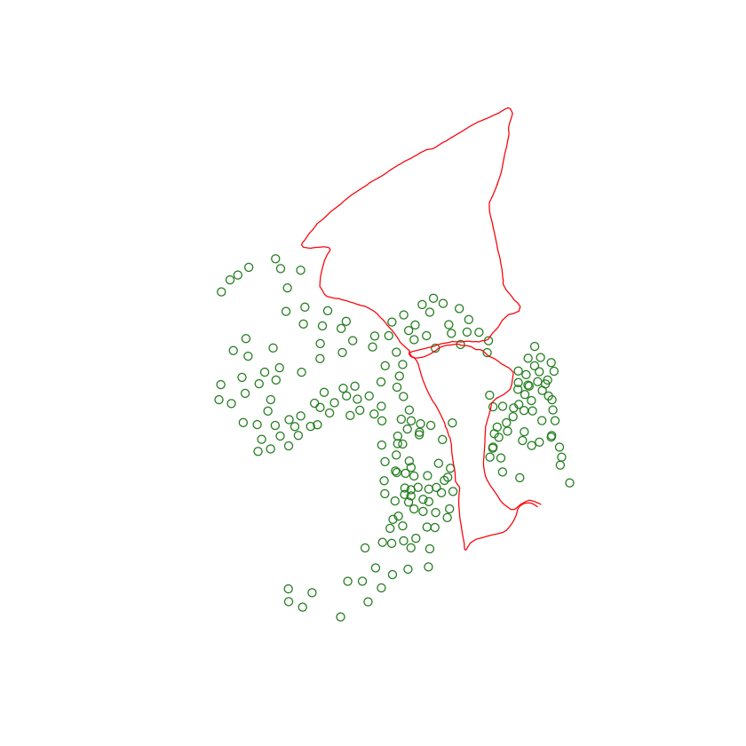

Plotting raster data¶

If you plot a raster object, it will plot each band separately:

# Plot the 3 bands of the silwood aerial image
names(silwood_aerial) <- c("Red", "Green", "Blue")
plot(silwood_aerial, nc=3)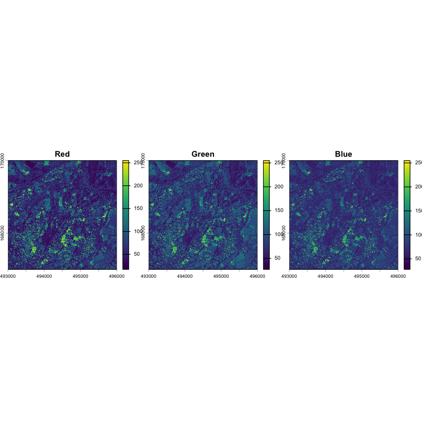

If you instead want to combine image bands to create a three colour image, then the terra::plotRGB can be used to combine 3 bands to generate a colour composite image. The silwood_aerial image contains the three RGB bands in the correct order, so we can simply plot it:

# Plot the silwood aerial data using the default settings
plotRGB(silwood_aerial)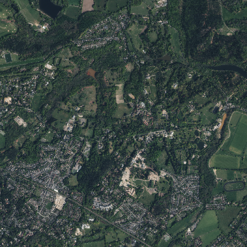

If we want to do the same thing with the RGB data from the Sentinel 2 data then we need to adjust the command to give the bands in the right order and also to set the maximum scale of the values across the bands.

# Plot the Sentinel data, setting the bands and scale
plotRGB(s2_silwood_10m, r=3, g=2, b=1, scale=0.80)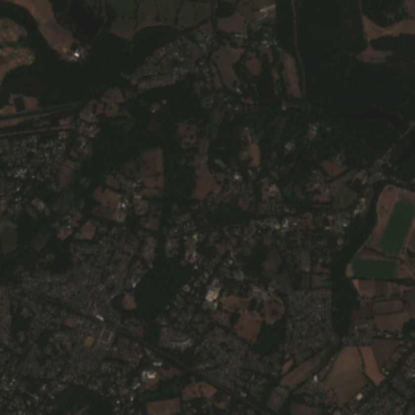

In fact, the L2A Sentinel 2 product provides a True Colour Image (TCI) that orders and scale the RGB bands to give something closer to expected colour. This can be used with the default settings.

# Load the L2A TCI image for Silwood and plot using defaults.
s2_silwood_tci <- rast(
  "../data/SpatialMethods/sentinel_2/R10m/silwood/T30UXC_20250711T110651_TCI_10m.tiff"
)
plotRGB(s2_silwood_tci)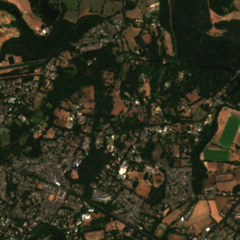

Alternatively, you can set different bands as inputs to give a “false-colour image”. One common usage is a false colour infrared image, which swaps from the [R, G, B] bands to [NIR, R, G]. This kind of imagery is very good at pulling out differences between vegetation (bright red), water (dark) and urban areas and bare ground (tan or grey).

# Plot the Sentinel data, setting the bands and scale
plotRGB(s2_silwood_10m, r=4, g=3, b=2, scale=0.8)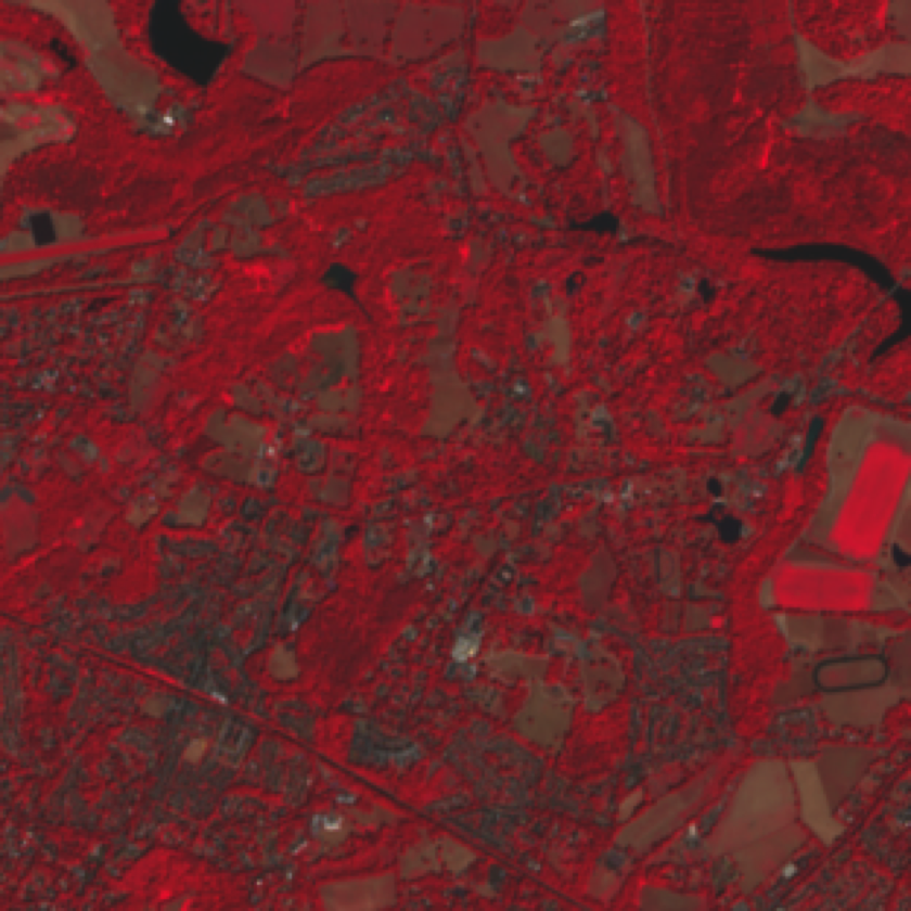

Reprojecting spatial data¶

We now have a large number of different datasets, but they are not all in the same GIS projection. We cannot use the datasets together until they use the same coordinate system. We will use the “OSGB 1936 / British National Grid” (or BNG) projection for all of the rest of the practical. It is a projected coordinate system, which means we can use metres to measure distances, and it is also the standard mapping system for the UK.

Reprojecting vector datasets¶

It is relatively easy to reproject vector datasets: all of the features in a vector dataset are built up from pairs of point. Reprojection is therefore just a matter of recalculating the coordinates in the new projection - the underlying equation might be complex but we are just moving points between two systems.

We can show the current range of coordinates for a dataset by looking at the extent of the data before.

# Show the extent of the sensor locations in the current WGS84 projection
ext(sensor_locations)

SpatExtent : -0.651972, -0.178122, 51.406849, 51.496483 (xmin, xmax, ymin, ymax)

The sf::st_transform function can then be used to transform data from one projection to another.

# Convert the WGS84 vector datasets to BNG
sensor_locations <- st_transform(sensor_locations, crs="EPSG:27700")
nest_boxes <- st_transform(nest_boxes, crs="EPSG:27700")
silmas_route <- st_transform(silmas_route, crs="EPSG:27700")

# Show the new extent
ext(sensor_locations)

SpatExtent : 493848.9919019, 526566.980292927, 168404.466202018, 179077.21373909 (xmin, xmax, ymin, ymax)

Reprojecting raster datasets¶

This is more involved than reprojecting vector data. You have a series of raster cell values in one projection and then want to insert representative values into a set of cells on a different projection. The borders of those new cells could have all sorts of odd relationships to the current ones.

We can show the issue by superimposing two grids:

A 200 m resolution grid using the extent of the BNG projection datasets for Silwood (red cells).
A very similar 200m grid taken from the extent of the Sentinel 2 data in the UTM30N projection for the same site and then reprojected into the BNG (grey cells)

# Create a BNG raster at 200m resolution for the study site
grid_BNG <- rast(ext(silwood_aerial), res = 200, crs = "EPSG:27700")
# Convert to an sf polygon dataset of grid cells
grid_BNG <- st_as_sf(as.polygons(grid_BNG))

# Create a UTM30N raster at 200 m resolution for the study site
grid_UTM30N <- rast(ext(s2_silwood_10m), res = 200, crs = "EPSG:32630")
# Convert to an sf polygon dataset _and_ then transform to BNG
grid_UTM30N <- st_as_sf(as.polygons(grid_UTM30N))
grid_UTM30N_in_BNG <- st_transform(grid_UTM30N, "EPSG:27700")

# Plot the two sets of grid cells over each other
plot(st_geometry(grid_UTM30N_in_BNG), reset=FALSE, border="grey")
plot(st_geometry(grid_BNG), border='red', add=TRUE)

# Add coordinates on the axes
axis(1)
axis(2)

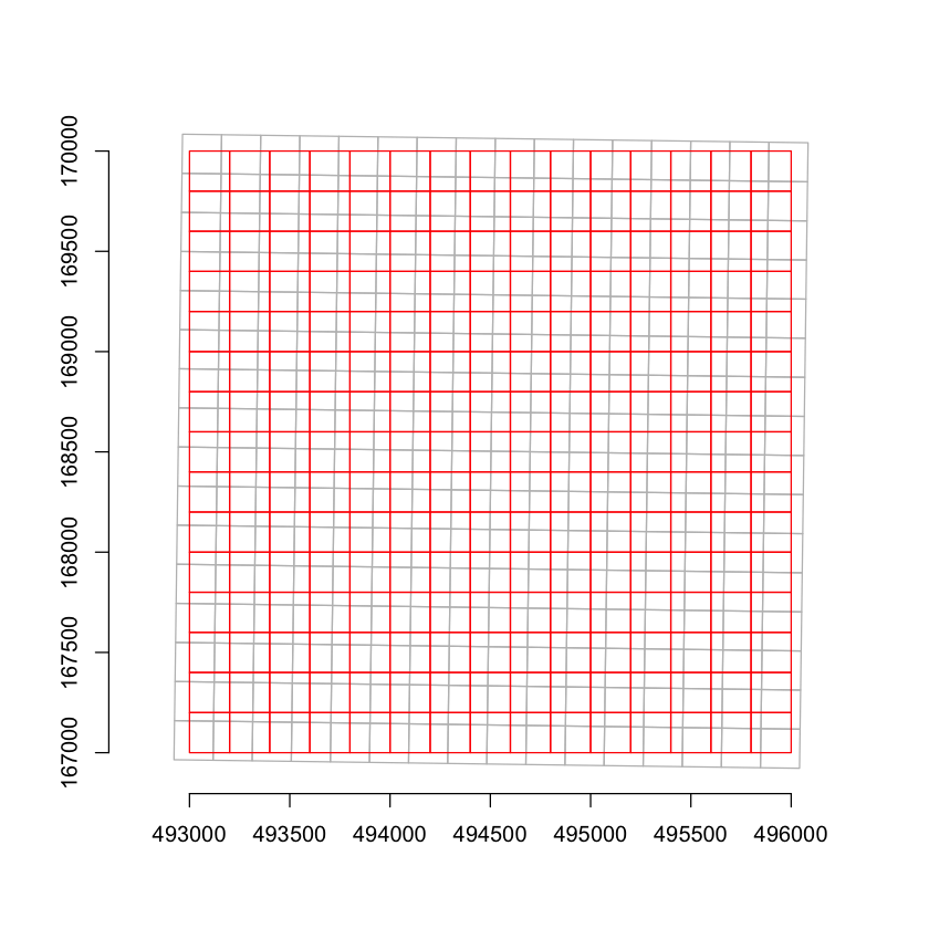
Plot source

In case you are interested in how the plot was created.

# Create a BNG raster at 200m resolution for the study site
grid_BNG <- rast(ext(silwood_aerial), res = 200, crs = "EPSG:27700")
# Convert to an sf polygon dataset of grid cells
grid_BNG <- st_as_sf(as.polygons(grid_BNG))

# Create a UTM30N raster at 200 m resolution for the study site
grid_UTM30N <- rast(ext(s2_silwood_10m), res = 200, crs = "EPSG:32630")
# Convert to an sf polygon dataset _and_ then transform to BNG
grid_UTM30N <- st_as_sf(as.polygons(grid_UTM30N))
grid_UTM30N_in_BNG <- st_transform(grid_UTM30N, "EPSG:27700")

# Plot the two sets of grid cells over each other
plot(st_geometry(grid_UTM30N_in_BNG), reset=FALSE, border="grey")
plot(st_geometry(grid_BNG), border='red', add=TRUE)

# Add coordinates on the axes
axis(1)
axis(2)

As you can see, even when the resolutions are the same, there is no neat one-to-one relationship between the two sets of cells: the axes of the two grids are not exactly parallel and the coordinates of the cell boundaries are not the same.

The terra::project function both converts the coordinates from one projection to another and resamples the data from one grid to another. There are various methods to carry out resampling - see the method details in ?project but they basically fall into two groups:

Most are interpolations methods for getting a representative continuous value for each cell from the data in the original raster grid. They range from simple average values of intersecting cells, to more complex polynomials and splines (e.g cubic) that use a moving window of a neighbourhood of cells to construct an estimate for the new cell.
Other approaches select a single value from the source grid: the near method takes the value from the source raster cell closest to the centre of the new cell, and the mode value takes the modal value of the set of overlapping cells. Both of these approaches are intended for use with categorical raster data, where it makes no sense to interpolate values between category codes.

To use the terra::project function, you need to provide a raster with the target resolution and projection to use as a template. To reproject the Sentinel 2 data, we can simply use the Land Cover map datasets, which are also have a 10m resolution and have been cropped to the study area.

s2_silwood_10m <- project(s2_silwood_10m, silwood_LCM, method="cubic")
s2_nhm_10m <- project(s2_nhm_10m, nhm_LCM, method="cubic")

Show solution

# Make 20 metre resolution templates for the study sites
silwood_template_20m <- rast(ext(silwood_aerial), res=20, crs="EPSG:27700")
nhm_template_20m <- rast(ext(nhm_aerial), res=20, crs="EPSG:27700")

# Reproject S2 20m bands into BNG
s2_silwood_20m <- project(s2_silwood_20m, silwood_template_20m, method="cubic")
s2_nhm_20m <- project(s2_nhm_20m, nhm_template_20m, method="cubic")

Manipulating raster data¶

Even once you have raster datasets in the same resolution, it is common to want to manipulate them to get multiple datasets into the same extent and resolution. This section covers:

upscaling and downscaling raster resolution,
joining adjacent raster tiles into a single dataset,
combining raster bands for datasets with the same extent and resolution, and
cropping datasets to a smaller extent.

Changing raster resolution¶

If you want to change the resolution or grid of an existing raster grid without changing the projection then you there are a few options:

If you want to change the grid resolution by a simple factor while keeping the same basic grid cell alignments and extent, then you can use the terra::aggregate and terra::disagg functions.
If you need to change the grid to a raster resolution that is not a simple factor or need to move the cell boundaries to match another dataset, then you will need the terra::resample function. This functions much like terra::project without the coordinate transformation, and has the same methods for resampling onto the new grid.

Here, we will use disaggregation to resample the 20 metre resolution Sentinel 2 bands to 10 metre resolution. We will use method=bilinear which uses a simple linear model to assign new cell values; the alternative method=near would simply duplicate the value from the nearest coarser resolution cell into each of the smaller cells.

s2_silwood_20m_at_10m <- disagg(s2_silwood_20m, fact=2, method="bilinear")
s2_nhm_20m_at_10m <- disagg(s2_nhm_20m, fact=2, method="bilinear")

We can use the terra::res function to show the resolutions of the two versions.

print(res(s2_silwood_20m))
print(res(s2_silwood_20m_at_10m))

[1] 20 20

[1] 10 10

Show solution

# It is actually very easy - we can just use the existing 10m CEH Land Cover Map
# datasets as the resampling template.
s2_silwood_20m_direct_to_10m <- project(
  s2_silwood_20m, silwood_lcm, method="cubic"
)
s2_nhm_20m_direct_to_10m <- project(
  s2_nhm_20m, nhm_lcm, method="cubic"
)

Mosaicing rasters¶

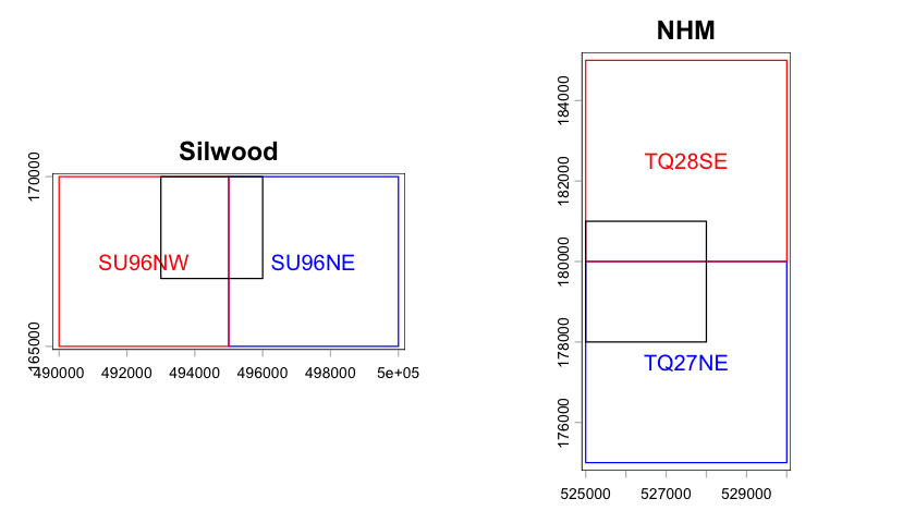
We can mosaic the two panes of Terrain 5 data for each site from two 5km panes into a single rectangle of data. The two panes are side by side for Silwood and one above the other for the NHM. The plot below shows the 5 x 5 km extent of the two panes. The figure also shows the 3 x 3 km extent of the other data sources - as you can see it overlaps the Terrain 5 panes for both sites, which is why we needed to load two panes.

options(repr.plot.height=4)

par(mfrow=c(1,2))

# Calculate the union of the extents of the two rasters
silwood_dtm_extent <- union(ext(silwood_dtm_SU96NE), ext(silwood_dtm_SU96NW ))

# Plot the extent of the first raster, but using the extent of both datasets
plot(ext(silwood_dtm_SU96NE), border="blue", ext=silwood_dtm_extent, main="Silwood")

# Get the middle coordinates of the raster and add a label. The `xFromCol` and 
# `yFromRow` functions extract the X and Y coordinates of cell centres from the 
# raster and `mean` then gives the centre of the raster image.
text(
  x=mean(xFromCol(silwood_dtm_SU96NE)), 
  y=mean(yFromRow(silwood_dtm_SU96NE)),
  labels="SU96NE", col="blue"
)

# Use `add=TRUE` to add the extent of the second raster and add the label
plot(ext(silwood_dtm_SU96NW), border="red", add=TRUE)
text(
  x=mean(xFromCol(silwood_dtm_SU96NW)), 
  y=mean(yFromRow(silwood_dtm_SU96NW)),
  labels="SU96NW", col="red"
)

# Finally add the extent of the other raster datasets 
plot(ext(silwood_aerial), border="black", add=TRUE)

# Repeat for the NHM datasets
nhm_dtm_extent <- union(ext(nhm_dtm_TQ27NE), ext(nhm_dtm_TQ28SE))

plot(ext(nhm_dtm_TQ27NE), border="blue", ext=nhm_dtm_extent, main="NHM")
text(
  x=mean(xFromCol(nhm_dtm_TQ27NE)), 
  y=mean(yFromRow(nhm_dtm_TQ27NE)),
  labels="TQ27NE", col="blue"
)
plot(ext(nhm_dtm_TQ28SE), border="red", add=TRUE)
text(
  x=mean(xFromCol(nhm_dtm_TQ28SE)), 
  y=mean(yFromRow(nhm_dtm_TQ28SE)),
  labels="TQ28SE", col="red"
)
plot(ext(nhm_aerial), border="black", add=TRUE)

Show source code for plot

The plot above uses a few useful plotting tricks for spatial data:

changing the spatial extent of the plot to include more than one dataset,
adding mutiple layers to a spatial plot, and
using coordinates to add text.

You do not need to know these details for the practical, but this might be something to come back to and look at.

options(repr.plot.height=4)

par(mfrow=c(1,2))

# Calculate the union of the extents of the two rasters
silwood_dtm_extent <- union(ext(silwood_dtm_SU96NE), ext(silwood_dtm_SU96NW ))

# Plot the extent of the first raster, but using the extent of both datasets
plot(ext(silwood_dtm_SU96NE), border="blue", ext=silwood_dtm_extent, main="Silwood")

# Get the middle coordinates of the raster and add a label. The `xFromCol` and 
# `yFromRow` functions extract the X and Y coordinates of cell centres from the 
# raster and `mean` then gives the centre of the raster image.
text(
  x=mean(xFromCol(silwood_dtm_SU96NE)), 
  y=mean(yFromRow(silwood_dtm_SU96NE)),
  labels="SU96NE", col="blue"
)

# Use `add=TRUE` to add the extent of the second raster and add the label
plot(ext(silwood_dtm_SU96NW), border="red", add=TRUE)
text(
  x=mean(xFromCol(silwood_dtm_SU96NW)), 
  y=mean(yFromRow(silwood_dtm_SU96NW)),
  labels="SU96NW", col="red"
)

# Finally add the extent of the other raster datasets 
plot(ext(silwood_aerial), border="black", add=TRUE)

# Repeat for the NHM datasets
nhm_dtm_extent <- union(ext(nhm_dtm_TQ27NE), ext(nhm_dtm_TQ28SE))

plot(ext(nhm_dtm_TQ27NE), border="blue", ext=nhm_dtm_extent, main="NHM")
text(
  x=mean(xFromCol(nhm_dtm_TQ27NE)), 
  y=mean(yFromRow(nhm_dtm_TQ27NE)),
  labels="TQ27NE", col="blue"
)
plot(ext(nhm_dtm_TQ28SE), border="red", add=TRUE)
text(
  x=mean(xFromCol(nhm_dtm_TQ28SE)), 
  y=mean(yFromRow(nhm_dtm_TQ28SE)),
  labels="TQ28SE", col="red"
)
plot(ext(nhm_aerial), border="black", add=TRUE)

We use the terra::mosaic function to combine these two panes into a single dataset for each site. There is also the terra::merge function: this is used to combine aligned raster datasets that are not simply neatly adjoining tiles. It also make life easier if we update these datasets so they use the same raster layer name - they currently are named by BNG grid pane.

# Mosaic the two Terrain 5 panes into a single dataset
silwood_dtm <- mosaic(silwood_dtm_SU96NE, silwood_dtm_SU96NW)
nhm_dtm <- mosaic(nhm_dtm_TQ27NE, nhm_dtm_TQ28SE)

# Update the raster layer names
names(silwood_dtm) <- names(nhm_dtm) <- "Elevation"

We can check the extents to show what happened - the new Silwood terrain dataset now has a 10km extent in the X dimension.

print(ext(silwood_dtm_SU96NE))
print(ext(silwood_dtm_SU96NW))
print(ext(silwood_dtm))

SpatExtent : 495000, 5e+05, 165000, 170000 (xmin, xmax, ymin, ymax)

SpatExtent : 490000, 495000, 165000, 170000 (xmin, xmax, ymin, ymax)

SpatExtent : 490000, 5e+05, 165000, 170000 (xmin, xmax, ymin, ymax)

Combining raster bands¶

We can also combine rasters with the same resolution and grid to add more bands onto an existing dataset. We can do this to create a new Sentinel 2 dataset that includes the original 10 metre resolution bands and the 20 metre bands that we resampled to 10 metres. The terra package takes the standard c() function for combining R vectors and lists and extends that to join raster layers by band.

# Combine the S2 10m bands with the resampled 20 m bands.
s2_silwood_10m <- c(s2_silwood_10m, s2_silwood_20m_at_10m)
s2_nhm_10m <- c(s2_nhm_10m, s2_nhm_20m_at_10m)

Cropping rasters¶

You can reduce the size of a raster dataset to a particular area of interest using the terra::crop function. We will use this to extract the 3km area of interest from the newly mosaiced datasets. All we need to provide is another dataset that has the required extent.

# Crop the mosaiced DTM data to the 3km area of interest.
silwood_dtm <- crop(silwood_dtm, silwood_aerial)
nhm_dtm <- crop(nhm_dtm, nhm_aerial)

We can again check the extents of the resulting grids to check that they match:

# Crop the mosaiced DTM data to the 3km area of interest.
print(ext(silwood_dtm))
print(ext(silwood_aerial))

SpatExtent : 493000, 496000, 167000, 170000 (xmin, xmax, ymin, ymax)

SpatExtent : 493000, 496000, 167000, 170000 (xmin, xmax, ymin, ymax)

Manipulating vector data¶

Vector data manipulation is generally either to merge two datasets or to crop data to a smaller spatial extent.

Merging vector data¶

Vector data is easier to merge in some ways: because the coordinates are recorded as sets of point forming features, you don’t have to worry about cell alignment or resolution. However, to merge a set of spatial features:

The two datasets have to have the same attributes: the data associated with each feature needs to match.
The two datasets have to be in the same projection.

Provided these two things are true, then merging two vector datasets is basically the same as binding together the rows of two data frames with the same structure. The sf package provides a version of the rbind function that joins two sf objects, and we can use this to combine the two VML panes for the sites.

# Combine the road panes
silwood_VML_roads <- rbind(vml_su96ne_roads, vml_su96nw_roads)
nhm_VML_roads <- rbind(vml_tq28se_roads, vml_tq27ne_roads)

# Combine the water area panes
silwood_VML_water <- rbind(vml_su96ne_water, vml_su96nw_water)
nhm_VML_water <- rbind(vml_tq28se_water, vml_tq27ne_water)

If we plot the extents of the new combined data (grey) and the source panes (red and blue) for Silwood, you can see that the panes are not neatly aligned with actual BNG grid cell bounds used by the elevation data (dashed panes). Raster cells by definition fall onto a neat grid, but vector features cross boundaries and it is common for datasets to include features that fall outside the strict pane boundaries.

# Merged data
plot(st_as_sfc(st_bbox(silwood_VML_roads)), border='grey', lwd=4)

# SU96NW panes of vector (solid) and raster (dashed) data
plot(st_as_sfc(st_bbox(vml_su96nw_roads)), border='blue', add=TRUE)
plot(st_as_sfc(st_bbox(silwood_dtm_SU96NW)), border='blue', add=TRUE, lty=2)

# SU96NE panes of vector (solid) and raster (dashed) data
plot(st_as_sfc(st_bbox(vml_su96ne_roads)), border='red', add=TRUE)
plot(st_as_sfc(st_bbox(silwood_dtm_SU96NE)), border='red', add=TRUE, lty=2)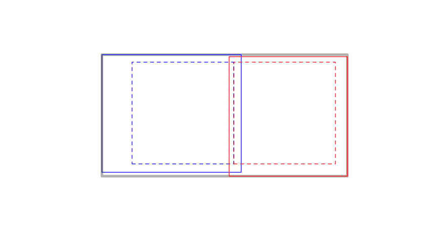

Cropping vector data¶

We can crop the VML data down to the study site using the sf::st_crop function. It is usually faster and easier to reduce datasets to only the focal area you are working with.

# Crop the two vector datasets
silwood_VML_roads <- st_crop(silwood_VML_roads, silwood_aerial)
nhm_VML_roads <- st_crop(nhm_VML_roads, nhm_aerial)
silwood_VML_water <- st_crop(silwood_VML_water, silwood_aerial)
nhm_VML_water <- st_crop(nhm_VML_water, nhm_aerial)

Warning message:
“attribute variables are assumed to be spatially constant throughout all geometries”

Warning message:
“attribute variables are assumed to be spatially constant throughout all geometries”

Warning message:
“attribute variables are assumed to be spatially constant throughout all geometries”

Warning message:
“attribute variables are assumed to be spatially constant throughout all geometries”

We can now create a simple plot overlaying the vector roads and water over the top of the digital elevations maps, again using sf::st_geometry to just show the geometries of the vector features.

par(mfrow=c(1, 2))

plot(silwood_dtm, col=grey.colors(20), main="Silwood")
plot(st_geometry(silwood_VML_roads), col="firebrick", add = TRUE)
plot(st_geometry(silwood_VML_water), col="cornflowerblue", border=NA, add = TRUE)

plot(nhm_dtm, col=grey.colors(20), main="NHM")
plot(st_geometry(nhm_VML_roads), col="firebrick", add = TRUE)
plot(st_geometry(nhm_VML_water), col="cornflowerblue", border=NA, add = TRUE)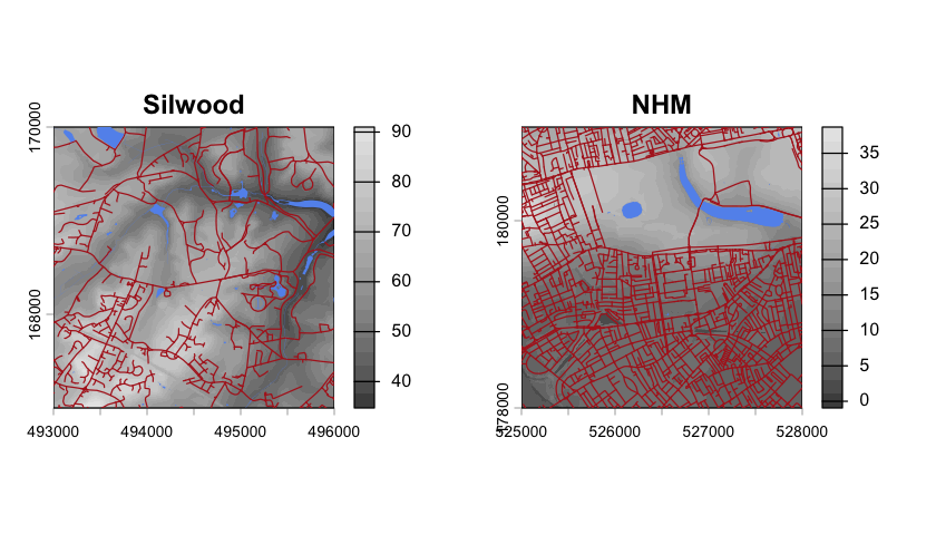

Raster calculations¶

A layer in a continuous raster dataset is basically just a large numeric matrix. This means you can use raster layers in equations to calulate new composite indices that emphasize different parts of the spectral signal. There are a very large number of remote sensing indices and the Sentinel-Hub scripts site provides formulae for a wide range of options. Here we will look at two simple vegetation indices.

NDVI¶

The normalised difference vegetation index (NDVI) is defined as:

NDVI = \frac{\text{NIR} - \text{RED}}{\text{NIR} + \text{RED}}

(1)

where NIR is band data for the near infrared and RED is band data in the red spectrum, which are Sentinel 2 bands B8 and B4. The index returns values from -1 (water) through 0 (rock and bare ground) to 1 (rainforest). See the Sentinel-Hub NDVI script page for more details.

# Calculate the NDVI index for the two sites
ndvi_nhm <- (
  s2_nhm_10m[["NIR"]] - s2_nhm_10m[["R"]]) / 
  (s2_nhm_10m[["NIR"]] + s2_nhm_10m[["R"]]
)
ndvi_silwood <- (
  s2_silwood_10m[["NIR"]] - s2_silwood_10m[["R"]]) / 
  (s2_silwood_10m[["NIR"]] + s2_silwood_10m[["R"]]
)
# Rename the single band 
names(ndvi_silwood) <- names(ndvi_nhm) <- "NDVI"

# Plot the NDVI index data
par(mfrow=c(1, 2))
plot(ndvi_silwood)
plot(ndvi_nhm)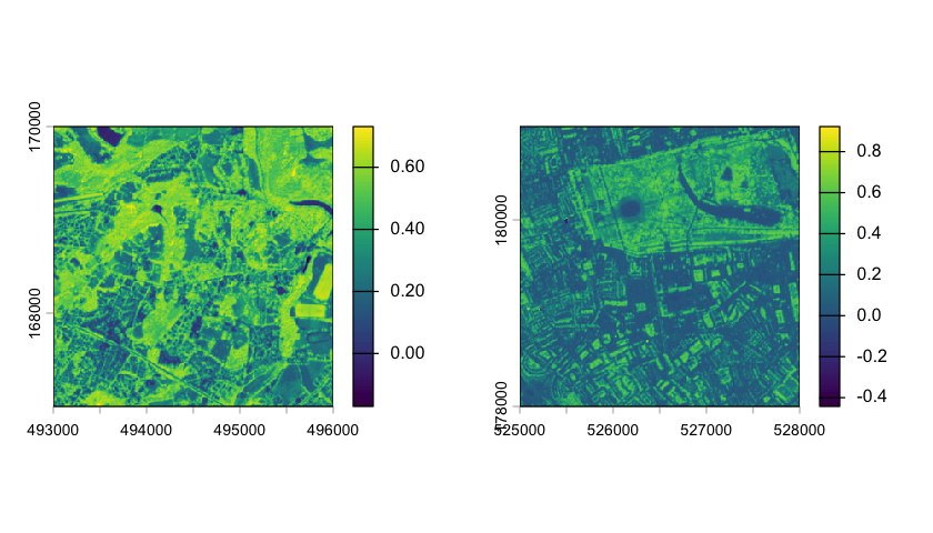

EVI¶

The enhanced vegetation index (EVI) is very similar but includes scaling factors and uses the Blue band (Sentinel B2) to improve how well the index captures vegetation. The scale again extends from -1 to 1. See the Sentinel-Hub EVI script page for more details.

EVI = 2.5 \cdot \left( \frac{\text{NIR} - \text{RED}} {\text{NIR} + 6 \cdot \text{RED} - 7.5 \cdot \text{BLUE} + 1} \right)

(2)

# Calculate the EVI index for the two sites
evi_nhm <- 2.5 * 
  (s2_nhm_10m[["NIR"]] - s2_nhm_10m[["R"]]) / 
  (s2_nhm_10m[["NIR"]] + 
    6 * s2_nhm_10m[["R"]] - 
    7.5 * s2_nhm_10m[["B"]] + 1)
  
evi_silwood <- 2.5 * 
  (s2_silwood_10m[["NIR"]] - s2_silwood_10m[["R"]]) / 
  (s2_silwood_10m[["NIR"]] + 
    6 * s2_silwood_10m[["R"]] - 
    7.5 * s2_silwood_10m[["B"]] + 1)

# Rename the single band 
names(evi_silwood) <- names(evi_nhm) <- "EVI"

There is an issue with the EVI data for the NHM site: there are some anomalous high values in the satellite data that lead to extreme EVI values. You can see these local issues as hotspots if you try plotting these bands (e.g. plot(s2_nhm_10m[["NIR"]])). We can fix that problem by setting extreme values to NA - this is another useful method for manipulating raster data.

# Remove anomalous EVI values
evi_nhm[evi_nhm > 1] <- NA
evi_nhm[evi_nhm < -1] <- NA

Now we can plot the EVI maps.

# Plot the EVI index data
par(mfrow=c(1, 2))
plot(evi_silwood)
plot(evi_nhm)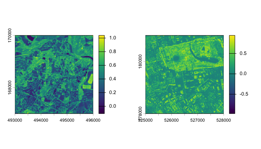

Sampling from raster datasets¶

A common need in spatial analysis is to get raster values from locations: for example, what are the EVI values at the nest box locations, or what are the heights of the sensor location sites. We can do this using the terra::extract function, which takes a raster and a vector dataset and returns the cell values under the vector features.

Point features¶

With point features this is very easy - you get the values under each point.

# Extract the EVI values under the nest boxes
nest_box_evi <- extract(evi_silwood, nest_boxes)
hist(nest_box_evi$EVI)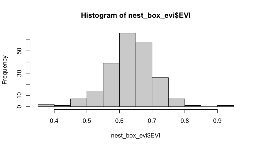

Plot with title “Histogram of nest_box_evi$EVI”

It is a little more difficult for the sensors because the heights are in two different datasets, so we need to use extract twice and then combine the results. The terra::extract function returns a row with NA if there is no data for a site, so we can merge the data simply by joining the two datasets together and dropping the NA rows.

# Extract the heights at the two sites
sensor_elevations_silwood <- extract(silwood_dtm, sensor_locations)
sensor_elevations_nhm <- extract(nhm_dtm, sensor_locations)

# Combine the values from the two rasters and drop to the combined data
sensor_elevations <- na.omit(rbind(sensor_elevations_silwood, sensor_elevations_nhm))

# Show the data
head(sensor_elevations)

Line features¶

You might also want to know what the values under a line feature are: either because you want a distribution of those values, or possible because you want a sequence of values along the feature. These two things are different - we’ll look at them using the Silmas walk/run route.

If we just use extract with the line features, then terra::extract returns the values of all of the cells that the line touches. The values are not in sequence along the line feature - they are just all the values it touches. We can see the cells that are being selected by rasterising the route.

# Extract the heights under the Silmas route
silmas_heights <- extract(silwood_dtm, silmas_route, xy=TRUE)

par(mfrow=c(1,2))
# Convert the Silmas route into a raster to show the sampled cells
silmas_route_raster <- rasterize(silmas_route, silwood_dtm)
plot(silwood_dtm, col=grey.colors(20))
plot(silmas_route_raster, col="red", add=TRUE, legend=FALSE)

# Show the height distribution of all the cells that the route crosses
hist(silmas_heights$Elevation, xlab = "Elevation of Silmas route cells (m)", main="")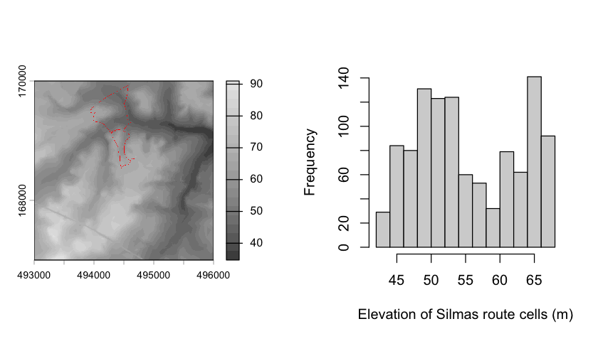

If you want to get a sequence of values along a linear feature then you need to extract the values in order. To do this, you need to convert the linear feature to points by casting it to the simpler feature type. This gives us a warning that basically just says that it is assigning the attributes for the whole linear feature to each and every point, and that might not be sensible. If the points are very spaced out, you can use sf::st_segmentize to interpolate more points along the feature.

silmas_points <- st_cast(silmas_route, "POINT")

Warning message in st_cast.sf(silmas_route, "POINT"):
“repeating attributes for all sub-geometries for which they may not be constant”

We can now use terra::extract on the points to get the heights in sequence. We can also use Pythagoras’ theorem to get the cumulative distance along the route from the coordinates.

# Get the height of each GPS point along the route
silmas_heights <- extract(silwood_dtm, silmas_points)

# Get the coordinates of the points and use Pythagoras to ge the distance.
coords <- as.data.frame(st_coordinates(silmas_points))
coords$distance <- c(0, sqrt(diff(coords$X)**2 + diff(coords$Y)**2))
coords$total_distance <- cumsum(coords$distance)
coords$height <-silmas_heights$Elevation

# Plot the height profile of the Silmas walk
plot(height~ total_distance, data=coords, type="l")

Polygon features¶

It is extremely common to want to get a distribution or summary statistic of raster values within a polygon feature: for example, what is the average elevation within 50 metres of each of the sensor locations? The first thing to do is to get polygons that form a 50m radius circle around each sensor locations using the sf::st_buffer function.

# Get 50m radius polygons around the sensor points
sensor_locations_50 <- st_buffer(sensor_locations, 50)

You can use sf::st_buffer with any features to get polygons extending out from the feature, and you can in fact use negative distances to get polygons within existing polygons. We can then use the polygon features with terra::extract to get a data frame of the values from the digital elevation map associated with each sensor location. We again need to join the results from the two sites together and drop any NA rows.

# Get the values within the 50m buffer for each sensor location, 
silwood_sensor_heights <- extract(silwood_dtm, sensor_locations_50)
nhm_sensor_heights <- extract(nhm_dtm, sensor_locations_50)
sensor_heights <- na.omit(rbind(silwood_sensor_heights, nhm_sensor_heights))

# How many values per site?
table(sensor_heights$ID)

# Height variation between sensors
boxplot(Elevation ~ ID, data= sensor_heights)


  1   2   3   4   5   6   7   8   9  10  11  12  13  14  15  16  17  18 
314 314 315 313 311 313 311 313 315 315 311 311 313 316 313 316 313 313

We can also extract data from categorical rasters:

# Get the values within the 50m buffer for each sensor location, 
silwood_sensor_LCM <- extract(silwood_LCM, sensor_locations_50)
nhm_sensor_LCM <- extract(nhm_LCM, sensor_locations_50)
sensor_LCM <- na.omit(rbind(silwood_sensor_LCM, nhm_sensor_LCM))

# Land cover class counts within 50m of each sensor.
xtabs(~ LandCover + ID, data= sensor_LCM, drop.unused.levels=TRUE)

                      ID
LandCover               1  2  3  4  5  6  7  8  9 10 11 12 13 14 15 16 17 18
  Broadleaved woodland 50 51 44 11 18  0 68 78 77 46 69 68  1 75  0  5  5  5
  Coniferous woodland   0 26  3  0  1  0  0  0  0  8  4  0  0  0  0  0  0  0
  Arable                0  0  0  0  0  0  0  0  0  0  0  0  0  0  1  1  2  2
  Improved grassland   19  0 11 66  0  0  7  0  0 13  0  9  0  4  0  0  0  0
  Neutral grassland     0  0  1  0  0  0  4  0  0  0  0  3  0  0  0  0  0  0
  Heather and shrub     2  1  0  0  0  0  0  0  0  2  1  0  0  0  0  0  0  0
  Freshwater            0  0 18  0  0  0  0  0  0  0  4  0  0  0  0  0  0  0
  Urban                 1  0  0  0  0 14  0  0  0  0  0  0 14  0 69 67 54 48
  Suburban              4  3  0  0 60 64  0  0  0  6  0  0 60  0  8  8 16 23

# Create an extent around a single sensor
zoom_to_site_one <- ext(c(493835,  493955, 169200, 169330))

# Rasterize using the two methods
cell_touches_false <- rasterize(sensor_locations_50[1,], silwood_dtm)
cell_touches_true <- rasterize(sensor_locations_50[1,], silwood_dtm, touches=TRUE)

# Plot side by side as DTM overplotted with rasterized polygon and polygon border
par(mfrow=c(1,2))

plot(
  silwood_dtm, ext=zoom_to_site_one, legend=FALSE, 
  col=gray.colors(20), main="touches=FALSE"
)
plot(cell_touches_false, add=TRUE, legend=FALSE, col="firebrick")
plot(st_geometry(sensor_locations_50[1,]), col=NA, add=TRUE)

plot(
  silwood_dtm, ext=zoom_to_site_one, legend=FALSE, 
  col=gray.colors(20), main="touches=TRUE"
)
plot(cell_touches_true, add=TRUE, legend=FALSE, col="firebrick")
plot(st_geometry(sensor_locations_50[1,]), col=NA, add=TRUE)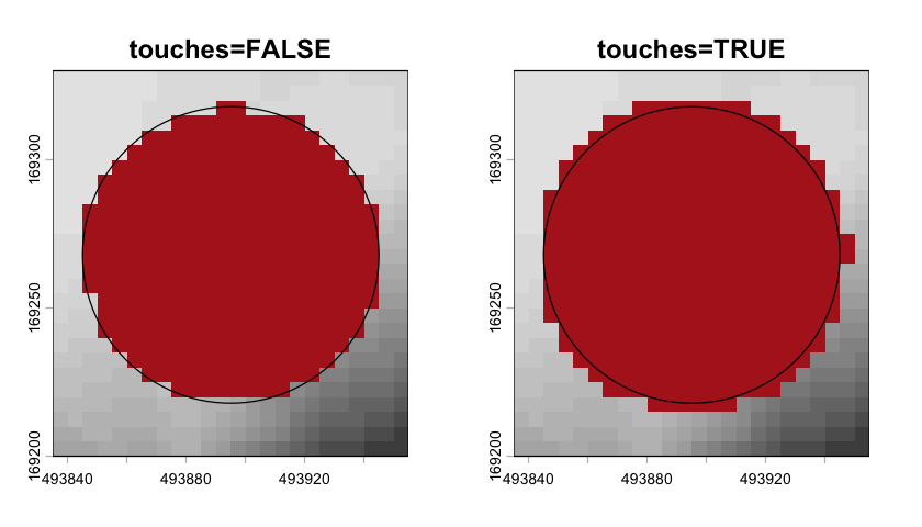

Zonal statistics¶

You can also sample from a raster dataset using another raster dataset. In practice, this is what is happening when you extract data from a vector feature - the different features get converted into raster layers in order to identify which cells to extract. But if you already have a categorical raster, you can simply use the terra::zonal function to extract the values under each raster cateogory.

# Extract the EVI values for each LCM raster cell
evi_by_LCM <- zonal(evi_silwood, silwood_LCM, wide=FALSE)
head(evi_by_LCM)

We can then visualise the range of EVI values by land cover class:

par(mar = c(4,12,1,1))
plot(EVI ~ as.factor(LandCover), data=evi_by_LCM, horizontal=TRUE, las=1, xlab="")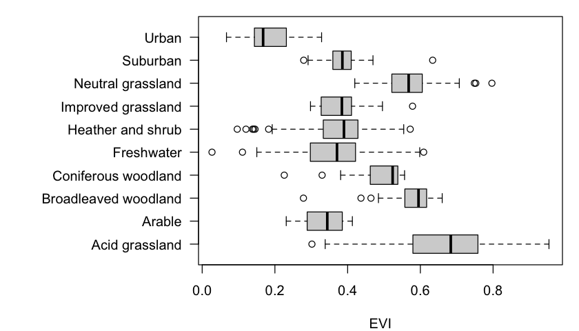

Image classification¶

We already have the CEH Land Cover map, but we may be able to get a better local model of land cover by classifying the Sentinel 2 data. Image classification is the process of taking spectral data from an image and identifying particular spectral signatures (combinations of values in the different bands) with a land cover category. You can classify simple RGB images, but it is often better to use data with more spectral bands: as we saw with the false colour infrared image, some bands are great at picking out particular features.

Unsupervised classification¶

Unsupervised classification tries to extract clusters of spectral signatures from the data. There are many approaches, but the basic aim of the algorithms is to try and find sets of points in the image that have similar spectral signatures.

Here we will use the base R stats::kmeans function to carry out k-means clustering on the data. The k of the k-means is the number of clusters we want to identify, and here we are letting the algorithm pick 10 random starting points from with the image spectra and then iterating to try and find stable sets of clusters. It then repeats that process with different starting choices and returns a classification across all of the runs.

# We need to convert the raster data into a data frame giving the 
# spectral signature of each cell
values <- as.data.frame(s2_silwood_10m)
head(values)

# Now we can run the clustering
n_cats <- 6
s2_kmeans <- kmeans(
  values, centers=n_cats, iter.max = 500, nstart = 5, algorithm="Lloyd"
)

# We can now take the cluster attribute from the output and put those values
# back into a 10m resolution raster
s2_kmeans_map <- rast(s2_silwood_10m, nlyr=1)
values(s2_kmeans_map) <- s2_kmeans$cluster

Now that we have the map, we can add labels and category names, as we did above for the CEH dataset.

labels <- data.frame(ID=1:n_cats, category=paste0("Category_", 1:n_cats))
#colours <- data.frame(ID=1:n_cats, colours=hcl.colors(n_cats, "Dark 2"))

colours <- data.frame(ID=1:n_cats, colours=carto_pal(n_cats, "Safe"))

levels(s2_kmeans_map) <- labels
coltab(s2_kmeans_map) <- colours

plot(s2_kmeans_map)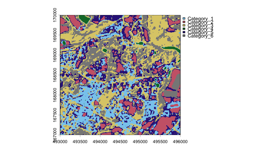

Supervised classification¶

The classes from an unsupervised classification are a purely statistical construction: they often do identify meaningful land cover types, but they need to be interpreted and it is common to re-run the process with different numbers of classes, or to merge classes that identify very similar regions.

The alternative of supervised classification avoids that by starting with a training dataset of sites with known categories. The spectral signatures of those sites can then be used to assign other sites to classes based on their similarity to the training data. This does mean that you need to put together a training dataset in one of two ways:

physically exploring the location with a GPS and assigning classes based on field data (“ground truthing”), or
selecting points from the imagery that visually belong to a particular class (“digitization”).

Here we use a training set drawn from inspecting the imagery, saved as a set of X and Y point coordinates and the land cover category at that point. There are multiple sites for each class, giving a distribution of signatures associated with each class.

# Load the classification data and convert it to an SF point dataset
training_sites <- read.csv("../data/SpatialMethods/S2_classification_data.csv")
training_sites <- st_as_sf(training_sites, coords=c("x","y"), crs="EPSG:27700")

# Plot the data over the top of an aerial image. This is a bit of a hack
# as it plots the vector data first to get the legend, then plots the aerial
# photo over the top and then the training sites _again_.
plot(training_sites, reset=FALSE)
plotRGB(silwood_aerial, add=TRUE)
plot(training_sites, add=TRUE)

# Show a table of the number of training sites for each category.
table(training_sites$category)


 Bare Ground    Grassland         Road Silwood Lake        Urban        Water 
           9           36           10            4           24            9 
    Woodland 
          37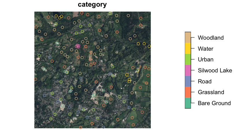

We can then extract the spectral signatures at each of those sites to give a spectral training dataset to use in classification.

# Extract a data frame of band values at each training site and add the
# category field to the dataset.
training_spectra <- extract(s2_silwood_10m, training_sites, ID=FALSE)
training_spectra$category <- training_sites$category

We will use a regression tree model using the rpart::rpart function to assign spectral signatures to classes. A regression tree finds critical values in the different bands that separate different classes and provides a simple decision tree based on the training data that can then be used to classify the whole image.

# Fit a regression tree of the land cover category as a function of the bands
s2_class_model <- rpart(
  category ~  B + G + R + NIR + RE5 + RE6 + RE7 + NNIR + SWIR1 + SWIR2,
  data = training_spectra, method = 'class', minsplit = 5
)

# Show the regression tree.
print(s2_class_model)

n= 129 

node), split, n, loss, yval, (yprob)
      * denotes terminal node

 1) root 129 92 Woodland (0.07 0.28 0.078 0.031 0.19 0.07 0.29)  
   2) R>=0.1304218 81 45 Grassland (0.11 0.44 0.099 0.049 0.3 0 0)  
     4) SWIR1>=0.356181 43  7 Grassland (0.12 0.84 0 0 0.047 0 0)  
       8) B>=0.2016674 3  0 Bare Ground (1 0 0 0 0 0 0) *
       9) B< 0.2016674 40  4 Grassland (0.05 0.9 0 0 0.05 0 0)  
        18) NIR>=0.3257478 38  2 Grassland (0.053 0.95 0 0 0 0 0) *
        19) NIR< 0.3257478 2  0 Urban (0 0 0 0 1 0 0) *
     5) SWIR1< 0.356181 38 16 Urban (0.11 0 0.21 0.11 0.58 0 0)  
      10) RE5< 0.2091596 12  5 Road (0 0 0.58 0.33 0.083 0 0)  
        20) RE6>=0.2886455 7  0 Road (0 0 1 0 0 0 0) *
        21) RE6< 0.2886455 5  1 Silwood Lake (0 0 0 0.8 0.2 0 0) *
      11) RE5>=0.2091596 26  5 Urban (0.15 0 0.038 0 0.81 0 0) *
   3) R< 0.1304218 48 11 Woodland (0 0 0.042 0 0 0.19 0.77)  
     6) NIR< 0.30421 10  1 Water (0 0 0.1 0 0 0.9 0) *
     7) NIR>=0.30421 38  1 Woodland (0 0 0.026 0 0 0 0.97) *

The model can then be used to predict values for all of the pixels. The resulting raster has one layer for each land cover type that gives the probability that the pixel is in that class.

# Generate the predictions for the whole map
s2_class_probability <- predict(s2_silwood_10m, s2_class_model)

# Plot 3 of the probability layers
plot(s2_class_probability[[1:3]], nc=3)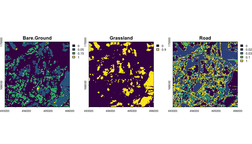

We can convert it into a land cover map by assigning each pixel to the class where it has the highest probability.

# Find the layer with the highest probability. The index of that code gives the 
# associated land  cover type
s2_class_map <- which.max(s2_class_probability)

# Assign level labels to the index codes.
levels(s2_class_map) <- data.frame(id=1:7, class=names(s2_class_probability))
plot(s2_class_map, col=carto_pal(7, "Safe"))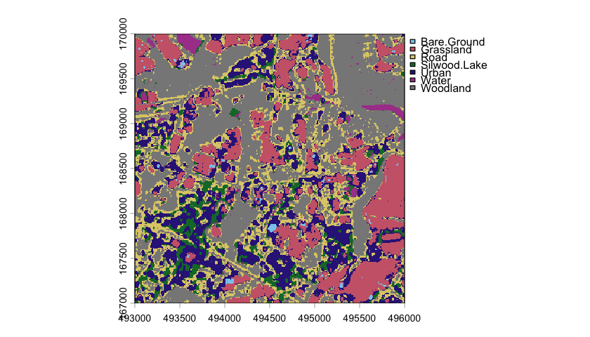

It is good practice to partition your training dataset to then test the accuracy of the classification - can your model successfully predict the classes of the data retained in the test partition. There are a lot of approaches to this (k-fold cross validation is a common one) but these are outside the scope of this practical.

Generating training data

Digitizing training data is one of those tasks where it may be easier to use a dedicated GIS program like GIS. This is mostly because it is easier to zoom in on an image to precisely place the training locations.

However, you can use R to create training datasets. The code below defines a function that can be used to generate a training data frame and then extend it with training data for different classes.

pick_training_sites <- function(category, df = NULL) {
    #' Function to add training data locations by clicking on a displayed map.
    #' 
    #' The function returns a data frame with the X and Y coordinates of the clicked
    #' points and a category field giving the `category` label for with the points.
    #' Press 'Escape' to finish collecting points and return a dataframe of coordinates.
    #' The returned dataframe for one category can be passed back into the `df`
    #' argument to append sites for a new category to the existing data. 

    # Pick the points from a plotted GIS map
    xy <- draw("points", pch=4)
    # Convert the selected coordinates to a dataframe and add the category label
    new_data <- as.data.frame(crds(xy))
    new_data$category <- category

    # Return the new_data appended to any existing data
    return(rbind(df, new_data))
}

# Plot the image
plotRGB(silwood_aerial)

# Build up the training set by clicking on the image and then pressing
# "escape" to finish defining one class and to move onto the next category
df <- pick_training_sites("Urban")
df <- pick_training_sites("Grassland", df=df)
df <- pick_training_sites("Water", df=df)
df <- pick_training_sites("Silwood Lake", df=df)
df <- pick_training_sites("Bare Ground", df=df)
df <- pick_training_sites("Woodland", df=df)
df <- pick_training_sites("Road", df=df)

# Export the data
write.csv(df, "../data/SpatialMethods/S2_classification_data.csv", row.names=FALSE)

Saving GIS files¶

# Remove any existing data output folder rather than have to stick a load of 
# overwrite=TRUE arguments in the student facing text.
if (dir.exists("spatial_method_practical_outputs")) {
  unlink("spatial_method_practical_outputs", recursive=TRUE)
}

We have created a lot of new dataset during this practical, which we should save for future use. The first thing to do is create a new directory to save the data files in:

# Create an output directory
dir.create("spatial_method_practical_outputs")
setwd("spatial_method_practical_outputs")

Saving raster data¶

We can write raster data out using the terra::writeRaster function. This function writes all the bands in the dataset out to a single file. The function uses the file suffix of the file name you provide to set the output format: there are lots of formats, but GeoTIFF is widely used and a good general choice.

# Create an output directory
dir.create("spatial_method_practical_outputs")
setwd("spatial_method_practical_outputs")

# Save the NDVI and EVI data
writeRaster(ndvi_silwood, "NDVI_Silwood.tiff")
writeRaster(ndvi_nhm, "NDVI_NHM.tiff")

writeRaster(evi_silwood, "EVI_Silwood.tiff")
writeRaster(evi_nhm, "EVI_NHM.tiff")

# Save the multiband Sentinel 2 data
writeRaster(s2_silwood_10m, "Sentinel2_Silwood.tiff")
writeRaster(s2_nhm_10m, "Sentinel2_NHM.tiff")

Saving vector data¶

The sf_st::write function is used to write vector data to file. Again, the file format is inferred from the output file name. This sf_st::write function is slightly more complex because file formats work in slightly different ways. The function has three main arguments:

obj: The sf object you want to write to a file.
dsn: The data source name that usually gives a filename that the data will be written to.
layer: A layer name within the data source that the data will be saved under. Not all formats support multiple layers (e.g. shapefiles), so you do not always need to provide a layer name.

There are many, many vector file formats - see the help file on sf::st_drivers() and the output

st_drivers()$name

The GeoPackage format is generally more convenient because it is a single file and can hold multiple layers. The code below saves the four processed VML subsets to a single GeoPackage file.

# Save the VML to GPKG
st_write(silwood_VML_roads, dsn="OS_VML_Silwood_NHM.gpkg", layer="silwood_VML_roads")
st_write(nhm_VML_roads, dsn="OS_VML_Silwood_NHM.gpkg", layer="nhm_VML_roads")
st_write(silwood_VML_water, dsn="OS_VML_Silwood_NHM.gpkg", layer="silwood_VML_water")
st_write(nhm_VML_water, dsn="OS_VML_Silwood_NHM.gpkg", layer="nhm_VML_water")

Writing layer `silwood_VML_roads' to data source 
  `OS_VML_Silwood_NHM.gpkg' using driver `GPKG'
Writing 780 features with 5 fields and geometry type Unknown (any).

Writing layer `nhm_VML_roads' to data source 
  `OS_VML_Silwood_NHM.gpkg' using driver `GPKG'
Writing 3154 features with 5 fields and geometry type Unknown (any).

Writing layer `silwood_VML_water' to data source 
  `OS_VML_Silwood_NHM.gpkg' using driver `GPKG'
Writing 113 features with 3 fields and geometry type Polygon.

Writing layer `nhm_VML_water' to data source 
  `OS_VML_Silwood_NHM.gpkg' using driver `GPKG'
Writing 37 features with 3 fields and geometry type Polygon.

Although the Shapefile format is more widely known, the inconvience of having multiple files is high and often leads to problems with incomplete datasets. It also has some odd constraints - as you can see in the output below, there is a limit to the length of attribute table field names in shapefiles.

# Save the sensors as shapefile
st_write(sensor_locations, dsn="sensor_locations.shp")

Warning message in abbreviate_shapefile_names(obj):
“Field names abbreviated for ESRI Shapefile driver”

Writing layer `sensor_locations' to data source 
  `sensor_locations.shp' using driver `ESRI Shapefile'
Writing 18 features with 24 fields and geometry type Point.