Course overview
Overview
Teaching: 5 min
Exercises: 0 minQuestions
What will this course cover?
In what lesson-style is this course delivered?
Objectives
Provide background information on course.
Overview
Programming as a researcher can be a very intimidating experience. It can feel as though your code isn’t “good enough” (as judged by some mysterious and opaque criteria), or that you’re not coding in the “right way”. The aim of this course is to help to address some of these concerns through an introduction to software engineering for researchers. Beyond just programming, software engineering is the practice and principle of writing software that is correct, sustainable and ready to share with colleagues and the wider research community.
Please, if you have not done so, yet, go through the setup instructions for the course.
Syllabus
- Techniques and tools to improve the readability and quality of your code
- Structuring your code in a modular fashion to promote reuse and future extension
- Testing frameworks and how to write tests
Learning Outcomes
On completion of this workshop you will be able to:
- Be confident in the quality of your code for collaboration and publication
- Apply appropriate quality assurance software tools to your code
- Write tests to check the correctness of your code
- Understand how and where to access support from the Research Computing Service at Imperial College
Delivery of the course
Material will be delivered as a lecture with tasks following the Carpentries teaching style.
- The instructor will walk you through the theoretical material of the course, demonstrating the execution of the relevant code and instructions. You are highly encouraged to code along and execute the instructions at the same time.
- Throughout the lessons, there are yellow boxes highlighting particularly challenging or important concepts.
- There are also exercises in orange boxes. The instructor will give you time to try to do them yourself before going through the solution. This is often available in a folded part of the orange box, so you can check it at any time.
- When doing exercises, put a green sticker in your computer whenever you are done, or a pink/orange one if you need support. A helper will go to you.
- For online sessions, raise your hand if you are done with the exercise and write any questions or problems directly into the chat, so a helper can try to solve it.
Key Points
Code along with the presenter.
Ask questions!
Tools I: Packaging and virtual-environments
Overview
Teaching: 5 min
Exercises: 10 minQuestions
How to use a package manager to install third party tools and libraries
Objectives
Use conda to install a reproducible environment
Python packages
- There are tens of thousands of python packages
- No need to reinvent the square wheel, it’s already out there
- Contributing to existing packages makes it more likely your work will be reused
- Contributing to open-source packages is the best way to learn how to code
Virtual environments
- Virtual environments isolate a project’s setup from the rest of the system
- It ensures different projects do not interfere with each other
- For instance, you may want simultaneously:
- a production environment with tried and true version of your software and tensorflow 1.15
- a development environment with shiny stuff and a migration to tensorflow 2.1
Package managers
Package managers help you install packages. Some help you install virtual environments as well. Better known python package managers include conda, pip, poetry
| conda | pip | poetry | |
|---|---|---|---|
| audience | research | all | developers |
| manage python packages | ✅ | ✅ | ✅ |
| manage non-python packages | ✅ | ❌ | ❌ |
| choose python version | ✅ | ❌ | ❌ |
| manage virtual envs | ✅ | ❌ | ✅ |
| easy interface | ❌ | ✅ | ❌ |
| fast | ❌ | ✅ | ✅ |
Package managers in other languages
- R: packrat and checkpoint
- C++: Conan and vcpkg
- Fortran: Fortran Package Manager (FPM)
Rules for choosing a package manager
- Choose one
- Stick with it
We chose conda because it is the de facto standard in science, and because it can natively install libraries such as fftw, vtk, or even Python, R, and Julia themselves.
It is also the de facto package manager on Imperial’s HPC cluster systems.
Example (10 min)
Installing and using an environment
If you haven’t already, see the setup guide for instructions on how to install Conda and Visual Studio Code.
Download this zip archive and extract it. Start Visual Studio Code and select “Open folder…” from the welcome screen. Navigate to the folder created from the archive and press “Select Folder”.
From the side-bar select the file
environment.yml. If you are prompted to install the Visual Studio Code Python extension then do so. The contents ofenvironment.ymlshould match:name: course dependencies: - python==3.11 - ruff - mypy - requestsCreate a new virtual environment using conda:
Windows users will want to open the app
Anaconda Promptfrom the Start Menu.Linux and Mac users should use a terminal app of their choice. You may see a warning with instructions. Please follow the instructions.
conda env create -f "path_to_environment.yml"You can obtain
path_to_environment.ymlby right clicking the file tab near the top of Visual Studio Code and selecting “Copy Path” from the drop-down menu. Make sure to include the quotation marks in the command. Right click on the window for your command line interface to paste the path.We can now activate the environment:
conda activate courseAnd check Python knows about the installed packages. Start a Python interpreter with the command
pythonthen:import requestsWe expect this to run without any messages. You can see the location of the installed package with:
requests.__file__'C:\\ProgramData\\Anaconda3\\envs\\course\\lib\\site-packages\\requests\\__init__.py'The file path you see will vary but note that it is within a directory called
coursethat contains all of the files for the virtual environment you have created. Exit the Python interpreter:exit()Finally, feel free to remove requests from
environment.yml, then runconda env update -f "path_to_environment.yml"and see whether the package has been updated or removed.
Solution
After completing step 7 you will find that the package has not been removed from the environment even after being removed from
environment.yml! If we runconda env update --helpwe get:usage: conda-env update [-h] [-n ENVIRONMENT | -p PATH] [-f FILE] [--prune] [--json] [-v] [-q] [remote_definition] Update the current environment based on environment file Options: positional arguments: remote_definition remote environment definition / IPython notebook optional arguments: -h, --help Show this help message and exit. -f FILE, --file FILE environment definition (default: environment.yml) --prune remove installed packages not defined in environment.ymlNotice the
--pruneoption. From the documentation it looks like we would need to runconda env update --prune -f "path_to_environment.yml". That flag is necessary to really uninstall unnecesary packages and update the environment. After running this command,import resquestwill fail.Note: If you are running
conda<23.9.0,import requestwill still work as there was a bug before that. You can check your conda version withconda --version.
Selecting an environment in Visual Studio Code
If you haven’t already, see the setup guide for instructions on how to install Visual Studio (VS) Code.
The simplest option for all platforms is to set the interpreter via the Command Palette:
- For Windows/Linux: Ctrl + Shift + P, and start typing “Python: Select interpreter”
- For macOS: Cmd + Shift + P, and start typing “Python: Select interpreter**
An entry should be present with the name course. It may take a few minutes
to appear however.
If you already have a Python file open then it’s also possible to set the interpreter using the toolbar at the bottom of the window.
Key Points
There are tens of thousands of Python packages
The choice is between reinventing the square wheel or reusing existing work
The state of an environment can be stored in a file
This stored environment is then easy to audit and recreate
Tools II: Code Formatters
Overview
Teaching: 5 min
Exercises: 5 minQuestions
How to format code with no effort on the part of the coder?
Objectives
Know how to install and use a code formatter
Why does formatting matter?
- Code is read more often than written
- It’s a menial task that adds cognitive load
- Ensures all code in a project is consistent, even if contributed by multiple authors
- Setting up a formatter in your editor takes 5 minutes
- Those 5 minutes are redeemed across the lifetime of the project
Rules to choose a code formatter
- Choose one
- Stick with it
We prefer ruff because it is modern, comprehensive
and runs very quickly. The ruff package is a collection of tools for ensuring
code quality in Python, including a code formatter and linter. We discuss its
formatter here, but will discuss the linter later as well.
A simpler alternative formatter is black, which has fewer options to fiddle with.
Formatters in other languages
- R: styler, with RStudio integration.
- C++: clang-format
- Fortran: findent and fprettify
Formatting example (5 min)
Using Visual Studio Code:
- Open the file
messy.py. Its contents should match:x = { 'a':37,'b':42, 'c':927} y = 'hello '+ 'world' class foo ( object ): def f (self ): z =3 return y **2 def g(self, x, # noqa: D102 y=42 ): return x--y def f ( a ) : return 37+-a[42-a : y*3]
- Ensure that you have activated your “course” conda environment (see previous episode)
- Make a trivial change to the file and save it: it should be reformatted automagically.
- Use the
undofunction of VS Code to return the code to its unformatted state. Before saving again delete a ‘:’ somewhere. When saving, the code will likely not format. It is syntactically invalid. The formatter cannot make sense of the code and thus can’t format it.Solution
After saving, the code should be automatically formatted to:
x = {"a": 37, "b": 42, "c": 927}
y = "hello " + "world"


class foo(object):
    def f(self):
        z = 3
        return y**2

    def g(
        self,
        x,  # noqa: D102
        y=42,
    ):
        return x - -y


def f(a):
    return 37 + -a[42 - a : y * 3]
Ah! much better! But note that the
# noqa: D102exclusion instruction is not in the right line and there’s a complain aboutgnot having a docstring.Still, the sharp-eyed user will notice at least one issue with this code. Formatting code does not make it less buggy!
Messy code exercise in Codespaces
If you are having trouble setting up your system with
condaandvscode, or running through this exercise locally in your computer, you can run it in Codespaces.
- Check the information at the end of the setup on how to run Codespaces.
- Apply it to this exercise repository in GitHub.
Key Points
Code formatting means how the code is typeset
It influences how easily the code is read
It has no impact on how the code runs
Almost all editors and IDEs have some means to set up an automatic formatter
5 minutes to set up the formatter is redeemed across the time of the project i.e. the cost is close to nothing
Tools III: Linters
Overview
Teaching: 5 min
Exercises: 10 minQuestions
How to make the editor pro-actively find errors and code-smells
Objectives
Remember how to install and use a linter in vscode without sweat
What is linting?
Linters enforce style rules on your code such as:
- disallow one letter variables outside of loops
- use
lower_snake_casefor variables - use
CamelCasefor classes - disallow nesting more than n deep
- detect code-smells (patterns that are often bugs, e.g. two functions with the same name)
- requiring all code to be appropriately documented
Consistent styles make a code more consistent and easier to read, whether or not you agree with the style. Using an automated linter avoids bike-shedding since the linter is the final arbiter.
Linters can also catch common errors such as:
- code that is never executed
- code with undefined behaviour
- variables that are never used
Why does linting matter?
- Code is read more often than written
- Ensures all code in a project is consistent, even if contributed by multiple authors
- Prevent simple bugs and mistakes
- Linters shortcut the
edit-run-debug and repeatworkflow - Setting up a linter in your editor takes 5 minutes
- Those 5 minutes are redeemed across the lifetime of the project
Rules for choosing linters
- Choose one or more
- Stick with them
We prefer ruff for fast and modern general linting.
ruff is also a great choice for a linter because it incorporates the checks of
multiple other linters, such as flake8 and pydocstyle, into a single tool.
You may also see these linters used by some projects:
- flake8 because it is simple
- pylint because it is (too?) extensive
- mypy for preventing type-related code errors
Checkout GitHub.com: Awesome Linters to see the range of linters available for different languages.
Linters in other languages
- R: lintr, with RStudio integration.
- C++: clang-tidy and CppCheck, although compilers can give lots of helpful linter-type warnings. For
gccandclang, it’s a good idea to pass the-Wall,-Wextraand-Wpedanticflags to get extra ones.- Fortran: fortran-linter and via compilers, like gfortran or Intel’s ifort and ifx
Exercise (10 min)
Setup VS Code:
- Return to
messy.py(now nicely formatted) in VS Code.- The output of the configured linters is shown displayed by coloured underlining in the editor, coloured vertical sections of the scroll bar and in the bottom status bar. Mouse over the underlined sections of the editor to see the reason for each.
- Check the current errors (click on errors in status bar at the bottom).
- Understand why each error is present and try to correct them.
- Alternatively, try and disable them (but remember: with great power…). We’ve already disabled-one at the function scope level. Check what happens if you move it to the top of the file at the module level.
Key Points
Linting is about discovering errors and code-smells before running the code
It shortcuts the “edit-run-debug and repeat” workflow
Almost all editors and IDEs have some means to setup automatic linting
5 minutes to setup a linter is redeemed across the time of the project i.e. the cost is close to nothing
Data Structures
Overview
Teaching: 30 min
Exercises: 25 minQuestions
How can data structures simplify codes?
Objectives
Understand why different data structures exist
Recall common data structures
Recognize where and when to use them
What is a data structure?
data structure: represents information and how that information can be accessed
Choosing the right representation for your data can vastly simplify your code and increase performance.
Choosing the wrong representation can melt your brain. Slowly.
Examples:
The number 2 is represented with the integer 2
>>> type(2)
int
Acceptable behaviors for integers include +, -, *, /
>>> 1 + 2
3
>>> 1 - 2
-1
On the other hand, text is represented by a string
>>> type("text")
str
It does not accept all the same behaviours as an integer:
>>> "a" + "b"
"ab"
>>> "a" * "b"
TypeError: can't multiply sequence by non-int of type 'str'
Integers can be represented as strings, but their behaviours would be unexpected:
>>> "1" + "2"
"12"
With integers, + is an addition, for strings it’s a concatenation.
Health impact of choosing the wrong data structure
- we could use
"1", "2", "3"to represent numbers, rather than1,2,3 -
we would have to reinvent how to add numbers, and multiply, and divide them e.g.
str(int("1") + int("2"))rather than just:
1 + 2 - the wrong data structures can make your code vastly more complicated
- also, the code would be much slower
Stay healthy. Stop and choose the right data structure for you!
Priorities for Choosing Data Structures
We’ve discussed how the incorrect data structure can make your code more complicated and also give worse performance. Quite often these two factors are aligned - the right data structure will combine simple code with the best performance. This isn’t always true however. In some cases simplicity and performance will be in tension with one another. A good maxim to apply here is “Premature optimization is the root of all evil”. This philosophy states that keeping your code simple and elegant should be your primary goal. Choosing a data structure based on performance or other considerations should only be considered where absolutely necessary.
Basic data structures
Different languages provide different basic structures depending on the purpose for which they were designed. We will consider here some of the basic data structures available in Python for which equivalents can be found in most other languages.
Lists
Lists are containers of other data:
# List of integers
[1, 2, 3]
# List of strings
["a", "b", "b"]
# List of lists of integers
[[1, 2], [2, 3]]
Lists make sense when:
- you have more than one item of data
-
the items are somehow related: Lists of apples and oranges are a code-smell
[1, 2, 3] # might be the right representation ["a", 2, "b"] # probably wrong -
the items are ordered and can be accessed
 >>> velocities_x = [0.3, 0.5, 0.1]
 >>> velocities_x[1]  # e.g. could be velocity a point x=1
Beware! The following might indicate a list is the wrong data structure:
- apples and oranges
- deeply nested list of lists of lists
Tuples
Python also has tuples which are very similar to lists. The main difference is that tuples are immutable which means that they can’t be altered after creation.
>>> a = ("a", "b")
>>> a[0] = "c"
Traceback (most recent call last):
  File "<stdin>", line 1, in <module>
TypeError: 'tuple' object does not support item assignment
Other languages
- C++:
- std::vector, fast read-write to element i and fast iteration operations. Slow insert operation.
- std::list. No direct access to element i. Fast insert, append, splice operations.
- R: list
- Julia: Array, also equivalent to numpy arrays.
- Fortran: array, closer to numpy arrays than python lists
Sets
Sets are containers where each element is unique:
>>> set([1, 2, 2, 3, 3])
{1, 2, 3}
They make sense when:
- each element in a container must be unique
-
you need to solve ownership issues, e.g. which elements are in common between two lists? Which elements are different?
  >>> set(["a", "b", "c"]).symmetric_difference(["b", "c", "e"])
  {'a', 'e'}
Something to bear in mind with sets is that, depending on your language, they may or may not be ordered. In Python sets are unordered i.e. the elements of a set cannot be accessed via an index, but sets in other languages may allow this.
Other languages
- C++: std::set
- R: set functions that operate on a standard list.
- Julia: Set
- Fortran: Nope. Nothing.
Dictionaries
Dictionaries are mappings between a key and a value (e.g. a word and its definition).
# mapping of animals to legs
{"horse": 4, "kangaroo": 2, "millipede": 1000}
They make sense when:
-
you have pairs of data that go together:
# A list of tuples?? PROBABLY BAD!! [ ("horse", "mammal"), ("kangaroo", "marsupial"), ("millipede", "alien") ] # Better? { "horse": "mammal", "kangaroo": "marsupial", "millipede": "alien" } -
given x you want to know its y: given the name of an animal you want to know the number of legs.
-
often used as bags of configuration options
Beware! The following might indicate a dict is the wrong data structure:
-
keys are not related to each other, or values are not related to each other
{1: "apple", "orange": 2}1not related to"orange"and2not related to"apple" -
deeply nested dictionaries of dictionaries of lists of dictionaries
Other languages
Basic Data Structure Practice (15 min)
You’re writing a piece of code to track the achievements of players of a computer game. You’ve been asked to design the data structures the code will use. The software will need the following data structures as either a list, a dictionary or a set:
- A collection containing all possible achievements
- A collection for each player containing their achievements in the order they were obtained (assume no duplicates)
- A collection relating player names to their achievements
You’re also told that the following operations on these datastructures will be needed:
- get a player’s achievements
- get a player’s first achievement
- add a new achievement for a player
- get the number of achievements a player doesn’t have yet
- get a collection of the achievements a player doesn’t have yet
- find the achievements “player1” has that “player2” doesn’t
Implement the data structures as seems most appropriate and populate them with some example data. Then have a go at writing code for some of the necessary operations. If you picked the right structures, each action should be able to be implemented as a single line of code.
Solution
all_achievements = {"foo", "bar", "baz"}

player_achievements = {
    "player1": ["foo", "baz"],
    "player2": [],
    "player3": ["baz"],
}

# get a player's achievements
player_achievements["player2"]

# get a player's first achievement
player_achievements["player1"][0]

# add a new achievement to a player's collection
player_achievements["player2"].append("foo")

# get the number of achievements a player doesn't have yet
len(all_achievements) - len(player_achievements["player2"])

# get a collection of the achievements a player doesn't have yet
all_achievements.difference(player_achievements["player1"])

# find the achievements player1 has that player2 doesn't
set(player_achievements["player1"]).difference(player_achievements["player2"])
Notice that for the last action we had to turn a list into a set. This isn’t a bad thing but if we were having to do it a lot that might be a sign we’d chosen an incorrect data structure.
Advanced data structures
Whilst basic data structures provide the fundamental building blocks of a piece of software, there are many more sophisticated structures suited to specialised tasks. In this section we’ll take a brief look at a variety of different data structures that provide powerful interfaces to write simple code.
Getting access to advanced data structures often involves installing additional libraries. As a rule of thumb, for any data structure you can think of somebody will already have published an implementation of it and its strongly recommended to use an available version rather than try to write one from scratch. We’ve discussed the best approach to managing dependencies for a project already.
Pandas Data Frames
The excellent and very powerful Panda’s package is the go to resource for dealing with tabular data. Anything you might think of using Excel for, Panda’s can do better. It leans heavily on NumPy for efficient numerical operations whilst providing a high level interface for dealing with rows and columns of data via pandas.DataFrame.
# working with tabular data in nested lists

data = [
    ["col1", "col2", "col3"],
    [0, 1, 2],
    [6, 7, 8],
    [0, 7, 8],
]

# get a single row or column
row = data[0]
col = [row[data[0].index("col1")] for row in data]

# filter out rows where col1 != 0
[data[0]] + [row for row in data[1:] if row[0] == 0]

# operate on groups of rows based on the value of col1
for val in set([row[0] for row in data[1:]]):
    rows = [row for row in data[1:] if row[0] == val]

# vs

import pandas as pd

# many flexible ways to create a dataframe e.g. import from csv, but here we
# use the use the existing data.
dataframe = pd.DataFrame(data[1:], columns=data[0])

# get a single row or column
row = dataframe.iloc[0]
col = dataframe["col1"]

# filter out rows where col1 != 0
dataframe[dataframe["col1"] == 0]

# operate on groups of rows based on the value of col1
dataframe.groupby("col1")
Balltrees
A common requirement across many fields is working with data points within a 2d, 3d or higher dimensioned space where you often need to work with distances between points. It is tempting in this case to reach for lists or arrays but balltrees provide an interesting and very performant alternative in some cases. An implementation is provided in Python by the scikit-learn library.
# Which point is closest to the centre of a 2-d space?

points = [
    [0.1, 0.1],
    [1.0, 0.1],
    [0.2, 0.2],
    [0.1, 0.3],
    [0.9, 0.2],
    [0.2, 0.3],
]
centre = [0.5, 0.5] # centre of our space

# Using lists

distances = []
for i, point in enumerate(points):
    dist = ((centre[0] - point[0])**2 + (centre[1] - point[1])**2)**0.5
    distances.append(dist)

smallest_dist = sorted(distances)[0]
nearest_index = distances.index(smallest_dist)

# vs

from sklearn.neighbors import BallTree

balltree = BallTree(points)
smallest_dist, nearest_index = balltree.query([centre], k=1)
Graphs and Networks
Another type of data structure that spans many different research domains are graphs/networks. There are many complex algorithms that can be applied to graphs so checkout the NetworkX library for its data structures.
edges = [
    [0, 1],
    [1, 2],
    [2, 4],
    [3, 1]
]

# Using lists

# get the degree (number of connected edges) of node 1

degree_of_1 = 0
for edge in edges:
    if 1 in edge:
        degree_of_1 += 1

# vs

import networkx as nx

graph = nx.Graph(edges)

# get the degree (number of connected edges) of node 1
graph.degree[1]

# easy to perform more advanced graph operations e.g.
graph.subgraph([1,2,4])
Custom data structures: Data classes
Python (>= 3.7) makes it easy to create custom data structures.
>>> from typing import List, Text
>>> from dataclasses import dataclass
>>> @dataclass
... class MyData:
...   a_list: List[int]
...   b_string: Text = "something something"
>>> data = MyData([1, 2])
>>> data
MyData(a_list=[1, 2], b_string='something something')
>>> data.a_list
[1, 2]
Data classes make sense when:
- you have a collections of related data that does not fit a more primitive type
- you already have a class and you don’t want to write standard functions like
__init__,__repr__,__ge__, etc..
Beware! The following might indicate a dataclass is the wrong data structure:
- you do need specialized
__init__behaviours (just use a class) - single huge mother of all classes that does everything (split into smaller specialized classes and/or stand-alone functions)
- a
dict,listornumpyarray would do the job. Everybody knows what anumpyarray is and how to use it. But even your future self might not know how to use your very special class.
Exploring data structures
Take some time to read in more detail about any of the data structures covered above or those below:
- deques
- named tuples
- counters
- dates
- enum represent objects that can only take a few values, e.g. colors. Often useful for configuration options.
- numpy arrays (multidimensional array of numbers)
- xarray arrays (multi-dimensional arrays that can be indexed with rich objects, e.g. an array indexed by dates or by longitude and latitude, rather than by the numbers 0, 1, 2, 3)
- xarray datasets (collections of named xarray arrays that share some dimensions.)
Don’t reinvent the square wheel.
Digital Oxford Dictionary, the wrong way and the right way (10 min)
Implement an oxford dictionary with two
lists, one for words, one for definitions:barf: (verb) eject the contents of the stomach through the mouth morph: (verb) change shape as via computer animation scarf: (noun) a garment worn around the head or neck or shoulders for warmth or decoration snarf: (verb) make off with belongings of others sound: | (verb) emit or cause to emit sound. (noun) vibrations that travel through the air or another medium surf: | (verb) switch channels, on television (noun) waves breaking on the shore- Given a word, find and modify its definition
- Repeat 1. and 2. with a
dictas the datastructure.- Create a subset dictionary (including definitions) of words rhyming with “arf” using either the two-
listor thedictimplementation- If now we want to also encode “noun” and “verb”, what data structure could we use?
- What about when there are multiple meanings for a verb or a noun?
Dictionary implemented with lists
def modify_definition(word, newdef, words, definitions):
    index = words.index(word)
    definitions = definitions.copy()
    definitions[index] = newdef
    return definitions


def find_rhymes(rhyme, words, definitions):
    result_words = []
    result_definitions = []
    for word, definition in zip(words, definitions):
        if word.endswith(rhyme):
            result_words.append(word)
            result_definitions.append(definition)
    return result_words, result_definitions


def testme():

    words = ["barf", "morph", "scarf", "snarf", "sound", "surf"]
    definitions = [
        "(verb) eject the contents of the stomach through the mouth",
        "(verb) change shape as via computer animation",
        (
            "(noun) a garment worn around the head or neck or shoulders for"
            "warmth or decoration"
        ),
        "(verb) make off with belongings of others",
        (
            "(verb) emit or cause to emit sound."
            "(noun) vibrations that travel through the air or another medium"
        ),
        (
            "(verb) switch channels, on television"
            "(noun) waves breaking on the shore"
        ),
    ]

    newdefs = modify_definition("morph", "aaa", words, definitions)
    assert newdefs[1] == "aaa"

    rhymers = find_rhymes("arf", words, definitions)
    assert set(rhymers[0]) == {"barf", "scarf", "snarf"}
    assert rhymers[1][0] == definitions[0]
    assert rhymers[1][1] == definitions[2]
    assert rhymers[1][2] == definitions[3]
Dictionary implemented with a dictionary
def modify_definition(word, newdef, dictionary):
    result = dictionary.copy()
    result[word] = newdef
    return result


def find_rhymes(rhyme, dictionary):
    return {
        word: definition
        for word, definition in dictionary.items()
        if word.endswith(rhyme)
    }


def testme():

    dictionary = {
        "barf": "(verb) eject the contents of the stomach through the mouth",
        "morph": "(verb) change shape as via computer animation",
        "scarf": (
            "(noun) a garment worn around the head or neck or shoulders for"
            "warmth or decoration"
        ),
        "snarf": "(verb) make off with belongings of others",
        "sound": (
            "(verb) emit or cause to emit sound."
            "(noun) vibrations that travel through the air or another medium"
        ),
        "surf": (
            "(verb) switch channels, on television"
            "(noun) waves breaking on the shore"
        ),
    }

    newdict = modify_definition("morph", "aaa", dictionary)
    assert newdict["morph"] == "aaa"

    rhymers = find_rhymes("arf", dictionary)
    assert set(rhymers) == {"barf", "scarf", "snarf"}
    for word in {"barf", "scarf", "snarf"}:
        assert rhymers[word] == dictionary[word]
More complex data structures for more complex dictionary
There can be more than one good answer. It will depend on how the dictionary is meant to be used later throughout the code.
Below we show three possibilities. The first is more deeply nested. It groups all definitions together for a given word, whether that word is a noun or a verb. If more often than not, it does not matter so much what a word is, then it might be a good solution. The second example flatten the dictionary by making “surf” the noun different from “surf” the verb. As a result, it is easier to access a word with a specific semantic category, but more difficult to access all definitions irrespective of their semantic category.
One pleasing aspect of the second example is that together things that are unlikely to change one one side (word and semantic category), and a less precise datum on the other (definitions are more likely to be refined).
The third possibility is a pandas
DataFramewith three columns. It’s best suited to big-data problems where individual words (rows) are seldom accessed one at a time. Instead, most operations are carried out over subsets of the dictionary.from typing import Text from enum import Enum, auto from dataclasses import dataclass from pandas import DataFrame, Series class Category(Enum): NOUN = auto VERB = auto @dataclass class Definition: category: Category text: Text first_example = { "barf": [ Definition( Category.VERB, "eject the contents of the stomach through the mouth" ) ], "morph": [ Definition( Category.VERB, "(verb) change shape as via computer animation" ) ], "scarf": [ Definition( Category.NOUN, "a garment worn around the head or neck or shoulders for" "warmth or decoration", ) ], "snarf": Definition(Category.VERB, "make off with belongings of others"), "sound": [ Definition(Category.VERB, "emit or cause to emit sound."), Definition( Category.NOUN, "vibrations that travel through the air or another medium", ), ], "surf": [ Definition(Category.VERB, "switch channels, on television"), Definition(Category.NOUN, "waves breaking on the shore"), ], } # frozen makes Word immutable (the same way a tuple is immutable) # One practical consequence is that dataclass will make Word work as a # dictionary key: Word is hashable @dataclass(frozen=True) class Word: word: Text category: Text second_example = { Word( "barf", Category.VERB ): "eject the contents of the stomach through the mouth", Word("morph", Category.VERB): "change shape as via computer animation", Word("scarf", Category.NOUN): ( "a garment worn around the head or neck or shoulders for" "warmth or decoration" ), Word("snarf", Category.VERB): "make off with belongings of others", Word("sound", Category.VERB): "emit or cause to emit sound.", Word( "sound", Category.NOUN ): "vibrations that travel through the air or another medium", Word("surf", Category.VERB): "switch channels, on television", Word("surf", Category.NOUN): "waves breaking on the shore", } # Do conda install pandas first!!! import pandas as pd third_example = pd.DataFrame( { "words": [ "barf", "morph", "scarf", "snarf", "sound", "sound", "surf", "surf", ], "definitions": [ "eject the contents of the stomach through the mouth", "change shape as via computer animation", ( "a garment worn around the head or neck or shoulders for" "warmth or decoration" ), "make off with belongings of others", "emit or cause to emit sound.", "vibrations that travel through the air or another medium", "switch channels, on television", "waves breaking on the shore", ], "category": pd.Series( ["verb", "verb", "noun", "verb", "verb", "noun", "verb", "noun"], dtype="category", ), } )
Key Points
Data structures are the representation of information the same way algorithms represent logic and workflows
Using the right data structure can vastly simplify code
Basic data structures include numbers, strings, tuples, lists, dictionaries and sets.
Advanced data structures include numpy array and panda dataframes
Classes are custom data structures
Structuring code
Overview
Teaching: 15 min
Exercises: 10 minQuestions
How can we create simpler and more modular codes?
Objectives
Explain the expression “separation of concerns”
Explain the expression “levels of abstractions”
Explain the expression “single responsibility principle”
Explain the expression “dataflow”
Analyze an algorithm for levels of abstractions, separable concerns and dataflow
Create focussed, modular algorithms
Structuring your code
Nutella Cake: What’s wrong in here?
Pour the preparation onto the dough. Wait for it to cool. Once it is cool, sprinkle with icing sugar.
The dough is composed of 250g of flour, 125g of butter and one egg yolk. It should be blind-baked at 180°C until golden brown.
The preparation consists of 200g of Nutella, 3 large spoonfuls of crème fraîche, 2 egg yolks and 20g of butter.
Add the Nutella and the butter to a pot where you have previously mixed the crème fraîche, the egg yolk and the vanilla extract. Cook and mix on low heat until homogeneous.
The dough, a pâte sablée, is prepared by lightly mixing by hand a pinch of salt, 250g of flour and 125g of diced butter until the butter is mostly all absorbed. Then add the egg yolk and 30g of cold water. The dough should look like coarse sand, thus its name.
Spread the dough into a baking sheet. If using it for a pie with a pre-cooked or raw filling, first cook the dough blind at 200°C until golden brown. If the dough and filling will be cooked together you can partially blind-cook the dough at 180°C for 15mn for added crispiness.
Enjoy! It’s now ready to serve!
Code is often as unreadable as this recipe, which makes things very hard to yourself and other people working on the code. Luckily, there are some rules and principles that can be followed to fix this and are a sign of good quality code.
In this lesson we will cover some of them, using the above recipe as an example, when relevant.
Separation of concerns
Separation of Concerns (SoC) is a fundamental design principle in software engineering that involves dividing a program into distinct sections, each addressing a separate concern. A concern is a specific aspect of functionality, behaviour, or responsibility within the system.
One of the first issues with the recipe above was that all the different elements were mixed up. The ingredients and the different steps of the preparation are all described together, making it impossible to figure out where to look to find out what to buy or how to prepare the dough or the filling.
Like the recipe, a piece of code should be split into multiple parts, each of them dealing with one aspect of the workflow. This makes the code more readable, and also more reusable, since the different parts could be mixed if their functionality were clearly separated.
For example, the following code will have clear separation of concerns along the whole workflow:
def main(filename, value):
  # reading input files is one thing
  data = read_input(filename)

  # creating complex objects is another
  simulator = Simulator(data)

  # compute is still something else
  result = simulator.compute(value)

  # Saving data is another
  save(result)
What concerns can you identify in the recipe?
Using the recipe above, what concerns can you identify? Concerns might be nested!
Solution
The first obvious separation could be between
IngredientsandPreparation. However, there is also another level betweenDoughandFilling, so a possible structure for the concerns could be:
- Ingredients
- Dough:
- …
- Filling:
- …
- Preparation
- Dough:
- …
- Filling:
- …
- Finishing
Solution 2
But there is another, more reusable solution, to separate the
Doughand theFillingfirst, and then theIngredientsand thePreparation. This way, the sameDoughcould be used in different cake recipes, and the same for theFilling.
- Dough
- Ingredients:
- …
- Preparation:
- …
- Filling
- Ingredients:
- …
- Preparation:
- …
- Finishing:
- Combine the dough and the filling prepared as above and…
Sometimes, there are multiple ways of separating the concerns, so spend some time upfront thinking on the simplest, yet more reusable solution for your code.
Levels of abstraction
Abstraction is a concept in computer science and software engineering that involves generalizing concrete details to focus on more important, generic aspects. It helps in managing complexity by hiding implementation details and exposing only the necessary parts.
Let’s consider the following code:
def analyse(input_path):
    data = load_data(input_path)

    # special fix for bad data point
    data[0].x["january"] = 0

    results = process_data(data)
    return results
The “special fix” mixes levels of abstraction. Our top level function now depends on
the structure of data. If the way data is stored changes (a low level detail) we
now also need to change analyse which is a high level function directing the flow
of the program.
The following code encapsulates those low level changes in another function, honouring the different levels of abstraction.
def analyse(input_path):
    data = load_data(input_path)

    cleaned_data = clean_data(data)

    results = process_data(cleaned_data)
    return results
Now our analyse function does not need to know anything about the inside workings
of the data object.
Single responsibility principle
The Single Responsibility Principle (SRP) states that a class or module should have only one reason to change, meaning it should have only one responsibility or purpose. This principle helps in creating more maintainable, reusable, and flexible software designs.
This goes into a deeper level than the abstractions described above, and it is probably the one harder to do right, besides its apparent simplicity. It literally means that each function or method should do one thing only. This typically means also that is short, easier to read, to debug and to re-use.
Let’s consider the following code. It uses Pandas to load some data from either an Excel file or a CSV file. In the second case, it also manipulates some columns to make sure the right ones are there.
def load_data(filename):
    if filename.suffix == ".xlsx":
        data = pd.read_excel(filename, usecols="A:B")

    elif filename.suffix == ".csv":
        data = pd.read_csv(filename)
        data["datetime"] = data["date"] + " " + data["time"]
        data = data.drop(columns=["date", "time"])

    else:
        raise RuntimeError("The file must be an Excel or a CSV file")

    assert data.columns == ["datetime", "value"]
    return data
This function is doing too many things despite being just 13 lines long, and might need to change for several, unrelated reasons. If we work on the separation of concerns, we will have several functions that:
- Select how to read the data based on the extension.
- Read an Excel file
- Read a CSV file
- Validate the data structure
def load_data(filename):
    """Select how to load the data based on the file extension."""
    if filename.suffix == ".xlsx":
        data = load_excel(filename)
    elif filename.suffix == ".csv":
        data = load_csv(filename)
    else:
        raise RuntimeError("The file must be an Excel or a CSV file.")
    return data

def load_excel(filename):
    """Loads an Excel file, picking only the first 2 columns."""
    data = pd.read_excel(filename, usecols="A:B")
    validate(data)
    return data

def load_csv(filename):
    """Loads a CSV file, ensuring the date and time are combined."""
    data = pd.read_csv(filename)
    data["datetime"] = data["date"] + " " + data["time"]
    data = data.drop(columns=["date", "time"])
    validate(data)
    return data

def validate(data):
    """Checks that the data has the right structure."""
    assert data.columns == ["datetime", "value"]
The overall length of the code is much more, but now each function does a very specific
thing, and only one thing, and well documented. The load_data function only needs to
change if more formats are supported. The load_excel only if the structure of the
Excel file changes and the same goes for the load_csv. And the validate data one, only
changes if there are more or different things to validate. The code becomes cleaner,
easier to read and to re-use.
Other considerations
Code legibility
Code is often meant to be read by an audience who has either not so much familiarity with it or has not work on it for a while. This audience is normally future-you reading past-you’s code.
For example, given a point with coordinates point[0], point[1], point[2], what do
each of them mean? Does 0 corresponds to x, y, or z? Or is it r, theta or
z? Or something else altogether?
Intelligible code aims to:
- Use descriptive names for variables and functions. The times where names should fit within 8 characters, and whole lines be less than 72 are long past.
- Avoid sources of confusion (What does index
0reference?) - Lessen the cognitive load (Before using
cdon’t forget to call the functionnothing_to_do_with_cbecause of historical implementation detail).
Some aspects of code legibility will be sorted - or at least flagged out - by the formatters and linters already discussed, but others do require a conscious effort by the developer.
Use of global variables
While global variables were common in the past, they have become less and less popular due to the problems they might bring to the code. Avoid the use global variables, when possible. They make the dataflow complex by essence.
Let’s consider the following code:
SOME_GLOBAL_VARIABLE = 42

def compute_a(measurements):
    ...
    result *= SOME_GLOBAL_VARIABLE
    return result
Now the result of compute_a has a hidden dependency. It’s never clear whether
calling it twice with the same input measurements will yield the same result, as
SOME_GLOBAL_VARIABLE might have changed.
In general make sure that all variables have the most limited scope possible. If they’re only needed within a single function define them there. Wherever possible treat variables with wide scope as constants (or make them actual constants if your language supports it) so you know they’re not being modified anywhere.
Having said that, there are situations where global variables are needed, or are just unavoidable. A typical example would be accessing a database. That database is just one of such global variables, accessible anywhere in the program, and might change in different places. There is no way around that, but just make sure that measures are in place to ensure that the state of the database is known at any given time.
Mixing IO and creating objects or making calculations
Input and output (IO) operations are tricky because they depend on the state of the system - the input file(s) contents - and change the state of the system - creating new file(s). They need to be handled with care and, indeed, some pure functional languages like Haskell consider them dirty operations because of that.
The general rule is that IO operations should happen within their own functions or methods, and and just pass their contents around. This is a direct conclusion of the Separation of concerns principle described above, as applied to IO operations.
For example, objects that need files to be created are hard to create and re-create, especially during testing. Make the contents of the file an input for the object creation function, instead of the filename or file object. You might want to use factory methods to support this approach.
For example, don’t do this:
class MyModel
    def __init__(self, some_array):
        self.some_array = array
        # BAD!! Now you need to carry this file around every time you want to
        # instantiate MyModel
        self.aaa = read_aaa("somefile.aaa")
Do this instead, so you can instantiate MyModel without having the file at hand:
class MyModel
    @classmethod
    def from_file(cls, array, filename):
        aaa = read_aaa(filename)
        return cls(array, aaa)

    def __init__(self, some_array, aaa):
        self.some_array = array
        self.aaa = aaa
Dataflow
Often code is just a sequence of transformations on data, so if we have the following set of actions:
- data
measurementsis read from input - data
aandbare produced frommeasurements, independently - data
resultis produced fromaandb
The code should reflect that structure:
def read_experiment(filename):
    ...
    return measurements

def compute_a(measurements):
    ...
    return a

def compute_b(measurements):
    ...
    return b

def compute_result(a, b):
    ...
    return result
- One function to read
Experiment - One function/class to compute
a: It takesmeasurementsas input and returns the resulta - One function/class to compute
b: It takesmeasurementsas input and returns the resultb - One function/class to compute
Result: It takesaandbas input and returns the resultresult:
Unnecessary arguments and tangled dependencies
What sometimes happens is that there are unnecessary arguments and tangled dependencies that can make the code harder to understand and, indeed, be a source of errors.
Look at the following alternative code:
# BAD! Unnecessary arguments. Now result depends on a, b, AND measurements
def compute_result(a, b, measurements):
    pass
Did we not say the result depends on a and b alone? The next programmer to look at
the code (e.g. future you) won’t know that. Computing result is no longer separate
from measurements.
Modifying an input argument
Some languages are designed so sometimes you don’t have any choice but to modify an input argument. Still, wherever possible avoid doing it because if you do not, other functions using that input argument will need to know who used it first!
If possible avoid doing this.
def compute_a(measurements):
    measurements[1] *= 2
    ...

def compute_b(measurements):
    some_result = measurements[1] * 0.5
    ...

def compute(measurements):
    compute_a(measurements)
    compute_b(measurements)
    ...
If compute_a takes place before compute_b the result would be different than if it
is the other way around. However, there is no clue in the compute function indicating
that is the case.
If you do need to modify the inputs then provide them as outputs of the function, such that it is clear by successive functions that they are using modified versions of the inputs.
def compute_a(measurements):
    measurements[1] *= 2
    ...
    return measurements

def compute_b(measurements):
    some_result = measurements[1] * 0.5
    ...
    return some_result

def compute(measurements):
    measurements = compute_a(measurements)
    some_result = compute_b(measurements)
    ...
Now it is clear that compute_b is using a measurements object that has been
outputted by compute_a and, therefore, it should expect any changes made by it.
Key Points
Code is read more often than written
The structure of the code should follow a well written explanation of its algorithm
Separate level of abstractions (or details) in a problem must be reflected in the structure of the code, e.g. with separate functions
Separable concerns (e.g. reading an input file to create X, creating X, computing stuff with X, saving results to file) must be reflected in the structure of the code
Testing Overview
Overview
Teaching: 15 min
Exercises: 5 minQuestions
Why test my software?
How can I test my software?
How much testing is ‘enough’?
Objectives
Appreciate the benefits of testing research software
Understand what testing can and can’t achieve
Describe various approaches to testing, and relevant trade-offs
Understand the concept of test coverage, and how it relates to software quality and sustainability
Appreciate the benefits of test automation
Why Test?
There are a number of compelling reasons to properly test a research code:
- Show that physical laws or mathematical relationships are correctly encoded
- Check that code works when running on a new system
- Make sure new code changes do not break existing functionality
- Ensure code correctly handles edge or corner cases
- Persuade others your code is reliable
- Check that code works with new or updated dependencies
Whilst testing might seem like an intimidating topic the chances are you’re already doing testing in some form. No matter the level of experience, no programmer ever just sits down and writes some code, is perfectly confident that it works and proceeds to use it straight away in research. Instead development is in practice more piecemeal - you generally think about a simple input and the expected output then write some simple code that works. Then, iteratively, you think about more complicated example inputs and outputs and flesh out the code until those work as well. When developers talk about testing all this means is formalising the above process and making it automatically repeatable on demand.
This has numerous advantages over a more ad hoc approach:
- Provides a record of the tests that have been carried out
- Faster development times - get feedback on changes quickly
- Encourages writing more modular code
- Ensures breakages are caught early in development
- Prevent manual testing mistakes
As you’re performing checks on your code anyway it’s worth putting in the time to formalise your tests and take advantage of the above.
A Hypothetical Scenario
Your supervisor has tasked you with implementing an obscure statistical method to use for some data analysis. Wanting to avoid unnecessary work you check online to see if an implementation exists. Success! Another researcher has already implemented and published the code.
You move to hit the download button, but a worrying thought occurs. How do you know this code is right? You don’t know the author or their level of programming skill. Why should you trust the code?
Now turn this question on its head. Why should your colleagues or supervisor trust any implementation of the method that you write? Why should you trust work you did a year ago? What about a reviewer for a paper?
This scenario illustrates the sociological value of automated testing. If published code has tests then you have instant assurance that its authors have invested time in the checking the correctness of their code. You can even see exactly the tests they’ve tried and add your own if you’re not satisfied. Conversely, any code that lacks tests should be viewed with suspicion as you have no record of what quality assurance steps have been taken.
Types of Testing
This isn’t a topic we will discuss in much detail but is worth mentioning as the jargon here can be another factor that is intimidating. In fact there are entire websites - even the Wikipedia - dedicated to explaining the different types of testing. Ultimately, however there are only a few types of testing that we need to worry about.
Unit Testing
The main type of testing kind we will be dealing with in this course. Unit testing refers to taking a component of a program and testing it in isolation. Generally this means testing an individual class or function. This is part of the reason that testing encourages more modular and sustainable code development. You’re encouraged to write your code into functionally independent components that can be easily unit tested.
Functional Testing
Unlike unit testing that focuses on independent parts of the system, functional testing checks the compliance of the system overall against a defined set of criteria. In other words does the software as a whole do what it’s supposed to do?
Regression Testing
This refers to the practice of running previously written tests whenever a new change is introduced to the code. This is good to do even when making seemingly insignificant changes. Carrying out regression testing allows you to remain confident that your code is functioning as expected even as it grows in complexity and capability.
Testing Done Right
It’s important to be clear about what software tests are able to provide and what they can’t. Unfortunately it isn’t possible to write tests that completely guarantee that your code is bug free or provides a one hundred percent faithful implementation of a particular model. In fact it’s perfectly possible to write an impressive looking collection of tests that have very little value at all. What should be the aim therefore when developing software tests?
In practice this is difficult to define universally but one useful mantra is that good tests thoroughly exercise critical code. One way to achieve this is to design test examples of increasing complexity that cover the most general case the unit should encounter. Also try to consider examples of special or edge cases that your function needs to handle especially.
A useful quantitative metric to consider is test coverage. Using additional tools it is possible to determine, on a line-by-line basis, the proportion of a codebase that is being exercised by its tests. This can be useful to ensure, for instance, that all logical branching points within the code are being used by the test inputs.
Testing and Coverage (5 min)
Consider the following Python function:
def recursive_fibonacci(n):
    """Return the n'th number of the fibonacci sequence"""
    if n <= 1:
        return n
    else:
        return recursive_fibonacci(n - 1) + recursive_fibonacci(n - 2)
Try to think up some test cases of increasing complexity, there are four distinct cases worth considering. What input value would you use for each case and what output value would you expect? Which lines of code will be exercised by each test case? How many cases would be required to reach 100% coverage?
For convenience, some initial terms from the Fibonacci sequence are given below: 0, 1, 1, 2, 3, 5, 8, 13, 21
Solution
Case 1 - Use either 0 or 1 as input
Correct output: Same as input Coverage: First section of if-block Reason: This represents the simplest possible test for the function. The value of this test is that it exercises only the special case tested for by the if-block.
Case 2 - Use a value > 1 as input
Correct output: Appropriate value from the Fibonacci sequence Coverage: All of the code Reason: This is a more fully fledged case that is representative of the majority of the possible range of input values for the function. It covers not only the special case represented by the first if-block but the general case where recursion is invoked.
Case 3 - Use a negative value as input
Correct output: Depends… Coverage: First section of if-block Reason: This represents the case of a possible input to the function that is outside of its intended usage. At the moment the function will just return the input value, but whether this is the correct behaviour depends on the wider context in which it will be used. It might be better for this type of input value to cause an error to be raised however. The value of this test case is that it encourages you to think about this scenario and what the behaviour should be. It also demonstrates to others that you’ve considered this scenario and the function behaviour is as intended.
Case 4 - Use a non-integer input e.g. 3.5
Correct output: Depends… Coverage: Whole function Reason: This is similar to case 3, but may not arise in more strongly typed languages. What should the function do here? Work as is? Raise an error? Round to the nearest integer?
Summary
The importance of automated testing for software development is difficult to overstate. As testing on some level is always carried out there is relatively low cost in formalising the process and much to be gained. The rest of this course will focus on how to carry out unit testing.
Key Points
Testing is the standard approach to software quality assurance
Testing helps to ensure that code performs its intended function: well-tested code is likely to be more reliable, correct and malleable
Good tests thoroughly exercise critical code
Code without any tests should arouse suspicion, but it is entirely possible to write a comprehensive but practically worthless test suite
Testing can contribute to performance, security and long-term stability as the size of the codebase and its network of contributors grows
Testing can ensure that software has been installed correctly, is portable to new platforms, and is compatible with new versions of its dependencies
In the context of research software, testing can be used to validate code i.e. ensure that it faithfully implements scientific theory
Unit (e.g. a function); Functional (e.g. a library); and Regression, (e.g. a bug) are three commonly used types of tests
Test coverage can provide a coarse- or fine-grained metric of comprehensiveness, which often provides a signal of code quality
Automated testing is another such signal: it lowers friction; ensures that breakage is identified sooner and isn’t released; and implies that machine-readable instructions exist for building and code and running the tests
Testing ultimately contributes to sustainability i.e. that software is (and remains) fit for purpose as its functionality and/or contributor-base grows, and its dependencies and/or runtime environments change
Writing unit tests
Overview
Teaching: 30 min
Exercises: 10 minQuestions
What is a unit test?
How do I write and run unit tests?
How can I avoid test duplication and ensure isolation?
How can I run tests automatically and measure their coverage?
Objectives
Implement effective unit tests using pytest
Execute tests in Visual Studio Code
Explain the issues relating to non-deterministic code
Implement fixtures and test parametrisation using pytest decorators
Configure git hooks and pytest-coverage
Apply best-practices when setting up a new Python project
Recognise analogous tools for other programming languages
Apply testing to Jupyter notebooks
Introduction
Unit testing validates, in isolation, functionally independent components of a program.
In this lesson we’ll demonstrate how to write and execute unit tests for a simple scientific code.
This involves making some technical decisions…
Test frameworks
We’ll use pytest as our test framework. It’s powerful but also user friendly.
For comparison: testing using assert statements:
from temperature import to_fahrenheit

assert to_fahrenheit(30) == 86
Testing using the built-in unittest library:
from temperature import to_fahrenheit
import unittest

class TestTemperature(unittest.TestCase):
    def test_to_farenheit(self):
        self.assertEqual(to_fahrenheit(30), 86)
Testing using pytest:
from temperature import to_fahrenheit

def test_answer():
    assert to_fahrenheit(30) == 86
Why use a test framework?
- Avoid reinventing the wheel - frameworks such as pytest provide lots of convenient features (some of which we’ll see shortly)
- Standardisation leads to better tooling, easier onboarding etc
Projects that use pytest:
Learning by example
Reading the test suites of mature projects is a good way to learn about testing methodologies and frameworks
Testing in other languages
- R: testthat
- C++: GoogleTest, Boost Test and Catch 2. See our C++ testing course using Google Test.
- Fortran: Test-Drive and pFUnit. See the Fibonacci series example coded in Fortran.
- See the Software Sustainability Institute’s Build and Test Examples for many more.
Code editors
We’ve chosen Visual Studio Code as our editor. It’s free, open source, cross-platform and has excellent Python (and pytest) support. It also has built-in Git integration, can be used to edit files on remote systems (e.g. HPC), and handles Jupyter notebooks (plus many more formats).
Demonstration of pytest + VS Code + coverage
- Test discovery, status indicators and ability to run tests inline
- Code navigation (“Go to Definition”)
- The Test perspective and Test Output
- Maximising coverage (
assert recursive_fibonacci(7) == 13)- Test-driven development: adding and fixing a new test (
test_negative_number)
A tour of pytest
Checking for exceptions
If a function invocation is expected to throw an exception it can be wrapped
with a pytest raises block:
def test_non_numeric_input():
    with pytest.raises(TypeError):
        recursive_fibonacci("foo")
Parametrisation
Similar test invocations can be grouped together to avoid repetition. Note how the parameters are named, and “injected” by pytest into the test function at runtime:
@pytest.mark.parametrize("number,expected", [(0, 0), (1, 1), (2, 1), (3, 2)])
def test_initial_numbers(number, expected):
    assert recursive_fibonacci(number) == expected
This corresponds to running the same test with different parameters, and is
our first example of a pytest decorator
(@pytest). Decorators
are a special syntax used in Python to modify the behaviour of the function,
without modifying the code of the function itself.
Skipping tests and ignoring failures
Sometimes it is useful to skip tests (conditionally or otherwise), or ignore failures (for example if you’re in the middle of refactoring some code).
This can be achieved using other @pytest.mark annotations e.g.
@pytest.mark.skipif(sys.platform == "win32", reason="does not run on windows")
def test_linux_only_features():
    ...

@pytest.mark.xfail
def test_unimplemented_code():
    ...
Refactoring
Code refactoring is “the process of restructuring existing computer code without changing its external behavior” and is often required to make code more amenable to testing.
Fixtures
If multiple tests require access to the same data, or a resource that is expensive to initialise, then it can be provided via a fixture. These can be cached by modifying the scope of the fixture. See this example from Devito:
@pytest.fixture
def grid(shape=(11, 11)):
    return Grid(shape=shape)

def test_forward(grid):
    grid.data[0, :] = 1.
    ...

def test_backward(grid):
    grid.data[-1, :] = 7.
    ...
This corresponds to providing the same parameters to different tests.
Tolerances
It’s common for scientific codes to perform estimation by simulation or other means. pytest can check for approximate equality:
def test_approximate_pi():
    assert 22/7 == pytest.approx(math.pi, abs=1e-2)
Random numbers
If your simulation or approximation technique depends on random numbers then consistently seeding your generator can help with testing. See
random.seed()for an example or the pytest-randomly plugin for a more comprehensive solution.
doctest
pytest has automatic integration with the Python’s standard
doctest module when invoked
with the --doctest-modules argument. This is a nice way to provide examples of
how to use a library, via interactive examples in
docstrings:
def recursive_fibonacci(n):
    """Return the nth number of the fibonacci sequence

    >>> recursive_fibonacci(7)
    13
    """
    return n if n <=1 else recursive_fibonacci(n - 1) + recursive_fibonacci(n - 2)
Hands-on unit testing (10 min)
Getting started
Setting up our editor
- If you haven’t already, see the setup guide for instructions on how to install Visual Studio Code and conda.
- Download and extract this zip file. If using an ICT managed PC please be sure to do this in your user area on the C: drive i.e.
C:\Users\your_username
- Note that files placed here are not persistent so you must remember to take a copy before logging out
- In Visual Studio Code go to File > Open Folder… and find the files you just extracted.
- If you see an alert “This workspace has extension recommendations.” click Install All and then switch back to the Explorer perspective by clicking the top icon on the left-hand toolbar
Open Anaconda Prompt (Windows), or a terminal (Mac or Linux) and run:
conda env create --file "path_to_environment.yml"The
path_to_environment.ymlcan be obtained by right-clicking the file name in the left pane of Visual Studio Code and choosing “Copy Path”. Be sure to include the quotation marks. Right click on the command line interface to paste.- Important: After the environment has been created go to View > Command Palette in VS Code, start typing “Python: Select interpreter” and hit enter. From the list select your newly created environment “diffusion”
Running the tests
- Open
test_diffusion.py- You should now be able to click on Run Test above the
test_heat()function and see a warning symbol appear, indicating that the test is currently failing. You may have to wait a moment for Run Test to appear.- Switch to the Test perspective by clicking on the flask icon on the left-hand toolbar. From here you can Run All Tests, and Show Test Output to view the coverage report (see Lesson 1 for more on coverage)
- Important: If you aren’t able to run the test then please ask a demonstrator for help. It is essential for the next exercise.
Diffusion exercise in Codespaces
If you are having trouble setting up your system with
condaandvscode, or running through this exercise locally in your computer, you can run it in Codespaces.
- Check the information at the end of the setup on how to run Codespaces.
- Apply it to this exercise repository in GitHub.
Advanced topics
More pytest plugins
pytest-benchmarkprovides a fixture that can transparently measure and track performance while running your tests:
def test_fibonacci(benchmark):
    result = benchmark(fibonacci, 7)
    assert result == 13
pytest-benchmark example
Demonstration of performance regression via recursive and formulaic approaches to Fibonacci calculation (output)
pytest-notebookcan check for regressions in your Jupyter notebooks (see also Jupyter CI)
- Hypothesis provides property-based testing, which is useful for verifying edge cases):
from fibonacci import recursive_fibonacci
from hypothesis import given, strategies

@given(strategies.integers())
def test_recursive_fibonacci(n):
    phi = (5 ** 0.5 + 1) / 2
    assert recursive_fibonacci(n) == int((phi ** n - -phi ** -n) / 5 ** 0.5)
Further resources
ImperialCollegeLondon/pytest_template_application- A tried-and-tested workflow for software quality assurance (repo)
- Using Git to Code, Collaborate and Share
- RCS courses and clinics
- Research Software Community
Key Points
Testing is not only standard practice in mainstream software engineering, it also provides distinct benefits for any non-trivial research software
pytest is a powerful testing framework, with more functionality than Python’s built-in features while still catering for simple use cases
Testing with VS Code is straightforward and encourages good habits (writing tests as you code, and simplifying test-driven development)
It is important to have a set-up you can use for every project - so that it becomes as routine in your workflow as version control itself
pytest has a myriad of extensions that are worthy of mention such as Jupyter, benchmark, Hypothesis etc
Unit Testing Challenge
Overview
Teaching: 10 min
Exercises: 50 minQuestions
How do I apply unit tests to research code?
How can I use unit tests to improve my code?
Objectives
Use unit tests to fix some incorrectly-implemented scientific code
Refactor code to make it easier to test
Introduction to your challenge
You have inherited some buggy code from a previous member of your research group: it has a unit test but it is currently failing. Your job is to refactor the code and write some extra tests in order to identify the problem, fix the code and make it more robust.
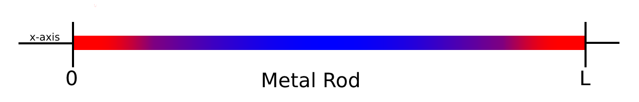
The code solves the heat equation, also known as the “Hello World” of Scientific Computing. It models transient heat conduction in a metal rod i.e. it describes the temperature at a distance from one end of the rod at a given time, according to some initial and boundary temperatures and the thermal diffusivity of the material:
The function heat() in diffusion.py attempts to implement a step-wise
numerical approximation via a finite difference
method:
This relates the temperature u at a specific location i and time point t
to the temperature at the previous time point and neighbouring locations. r is
defined as follows, where α is the thermal diffusivity:
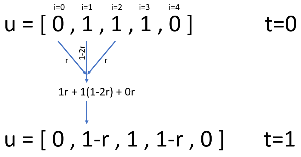
We approach this problem by representing u as a Python list. Elements within
the list correspond to positions along the rod, i=0 is the first element,
i=1 is the second and so on. In order to increment t we update u in a
loop. Each iteration, according to the finite difference equation above, we
calculate values for the new elements of u.
The test_heat() function in test_diffusion.py compares this approximation
with the exact (analytical) solution for the boundary conditions (i.e. the
temperature of the end being fixed at zero). The test is correct but failing -
indicating that there is a bug in the code.
Testing (and fixing!) the code (50 min)
Work by yourself or with a partner on these test-driven development tasks. Don’t hesitate to ask a demonstrator if you get stuck!
Separation of concerns
First we’ll refactor the code, increasing its modularity. We’ll extract the code that performs a single time step into a new function that can be verified in isolation via a new unit test:
In
diffusion.pymove the logic that updatesuwithin the loop in theheat()function to a new top-level function:def step(u, dx, dt, alpha): …Hint: the loop in
heat()should now look like this:for _ in range(nt - 1): u = step(u, dx, dt, alpha)- Run the existing test to ensure that it executes without any Python errors. It should still fail.
Add a test for our new
step()function:def test_step(): assert step(…) == …It should call
step()with suitable values foru(the temperatures at timet),dx,dtandalpha. It shouldassertthat the resulting temperatures (i.e. at timet+1) match those suggested by the equation above. Useapproxif necessary. _Hint:step([0, 1, 1, 0], 0.04, 0.02, 0.01)is a suitable invocation. These values will giver=0.125. It will return a list of the form[0, ?, ?, 0]. You’ll need to calculate the missing values manually using the equation in order to compare the expected and actual values.- Assuming that this test fails, fix it by changing the code in the
step()function to match the equation - correcting the original bug. Once you’ve done this all the tests should pass.Solution 1
Your test should look something like this:
# test_diffusion.py
def test_step():
    assert step([0, 1, 1, 0], 0.04, 0.02, 0.01) == [0, 0.875, 0.875, 0]
Your final (fixed!)
step()function should look like this. The original error was a result of some over-zealous copy-and-pasting.# diffusion.py def step(u, dx, dt, alpha): r = alpha * dt / dx ** 2 return ( u[:1] + [ r * u[i + 1] + (1 - 2 * r) * u[i] + r * u[i - 1] for i in range(1, len(u) - 1) ] + u[-1:] )
Now we’ll add some further tests to ensure the code is more suitable for publication.
Testing for exceptions
We want the
step()function to raise an Exception when the following stability condition isn’t met:Add a new test
test_step_unstable, similar totest_stepbut that invokesstepwith analphaequal to0.1and expects anExceptionto be raised. Check that this test fails before making it pass by modifyingdiffusion.pyto raise anExceptionappropriately.Solution 2
# test_diffusion.py
def test_step_unstable():
    with pytest.raises(Exception):
        step([0, 1, 1, 0], 0.04, 0.02, 0.1)

# diffusion.py
def step(u, dx, dt, alpha):
    r = alpha * dt / dx ** 2

    if r > 0.5:
        raise Exception

    …
Adding parametrisation
Parametrise
test_heat()to ensure the approximation is valid for some other combinations ofLandtmax(ensuring that the stability condition remains true).Solution 3
# test_diffusion.py
@pytest.mark.parametrize("L,tmax", [(1, 0.5), (2, 0.5), (1, 1)])
def test_heat(L, tmax):
    nt = 10
    nx = 20
    alpha = 0.01

    …
After completing these two steps check the coverage of your tests via the Test Output panel - it should be 100%.
The full, final versions of diffusion.py and test_diffusion.py are available on GitHub.
Bonus tasks
- Write a doctest-compatible docstring for
step()orheat()- Write at least one test for our currently untested
linspace()function
- Hint: you may find inspiration in numpy’s test cases, but bear in mind that its version of linspace is more capable than ours.
Key Points
Writing unit tests can reveal issues with code that otherwise appears to run correctly
Adding unit tests can improve software structure: isolating logical distinct code for testing often involves untangling complex structures
pytest can be used to add simple tests for python code but also be leveraged for more complex uses like parametrising tests and adding tests to docstrings
Advanced Topic: Design Patterns
Overview
Teaching: 30 min
Exercises: 30 minQuestions
How can we avoid re-inventing the wheel when designing code?
How can we transfer known solutions to our code?
Objectives
Recognize much-used patterns in existing code
Re-purpose existing patterns as solutions to new problems
What is a design pattern?
software design patterns: typical solutions to common problems
Pros
- It is easier to reuse known solutions than to invent them
- Makes the code easier to understand for collaborators
- Makes the code easier to maintain since patterns ought to be best-in-class solutions
Cons
- Shoehorning: not all patterns fit everywhere
- Patterns paper-over inadequacies that exist in one language but not another
- the visitor pattern is popular in Java or C++, but useless in Julia, thanks to multiple dispatch
- Haskell’s functional style makes the strategy pattern so obvious, it’s not longer a pattern, it’s the way things are done
Examples:
- Iterator pattern (see below) separates how to loop from what to do in a loop
- Dependency injection (see below) makes it easier to create modular algorithms
- Resource allocation is acquisition idiom promotes creating fully functional objects in one go
- Factory pattern separates creating object from the class of the object. It is used to unify or simplify the creation of similar objects into a single function.
- Adapter pattern interfaces one class to be used in an another
- More and more and more patterns
- And let’s not forget anti-patterns, i.e. patterns that should not be used
Resources
There are plenty of resources out there that you can follow to better understand design patterns. Here you have a couple that we have found useful:
- Refactoring.guru: Page with general description of patterns, with pseudocode, applicable to any programming language. It also has a section on (surprise!) refactoring your code.
- Design patterns in Python: Series of blog posts on the application of several design patterns in Python specifically, with example code.
Iterator Pattern
Iterators separates generating items over which to loop from doing the body of the loop. It separates looping from computing.
For instance, we want to loop over all items in xs and ys:
for x in xs:
    for y in ys:
        compute(x, y)
The code above can be transformed to:
from itertools import product

for x, y in product(xs, ys):
    compute(x, y)
Behind the scenes,
itertool’s product
returns an
iterator, i.e.
something we can loop over.
Using product is both simpler and more general. Now the number of nested loops
can be determined at runtime. It is no longer hard-coded.
>>> from itertools import product
>>> list_of_lists = [[1, 2], [3, 4]]
>>> for args in product(*list_of_lists):
...     print(args)
(1, 3)
(1, 4)
(2, 3)
(2, 4)
>>> list_of_lists = [[1, 2], [3, 4], [5, 6]]
>>> for args in product(*list_of_lists):
...     print(args)
(1, 3, 5)
(1, 3, 6)
(1, 4, 5)
(1, 4, 6)
(2, 3, 5)
(2, 3, 6)
(2, 4, 5)
(2, 4, 6)
Generators: iterators made easy
Generators create iterators using syntax that is similar to the standard loop:
for x in xs:
    for y in ys:
        print(f"some complicated calculation with {x} and {y}")
We can lift the loops out of the code and create a generator:
def my_generator(xs, ys):
  for x in xs:
      for y in ys:
          yield x, y
          print(f"I am in my_generator {x}, {y}")
And then loop with an iterator which python creates auto-magically:
>>> for x, y in my_generator([1, 2], ["a", "b"]):
...     print(f"some complicated calculation with {x} and {y}")
some complicated calculation with 1 and a
I am in my_generator 1, a
some complicated calculation with 1 and b
I am in my_generator 1, b
some complicated calculation with 2 and a
I am in my_generator 2, a
some complicated calculation with 2 and b
I am in my_generator 2, b
In practice, Python runs through the code in my_generator and returns a new
element each time it hits yield. The next time it is called, it restarts from
the line right after yield.
When to use generators?
- To separate complex loops from complex calculations in the loop
- Complex loops that occur multiple times in the code (copy-paste is a foot gun).
- When running out of memory, generators allow you be lazy
- Use iterators when the language does not allow for generators (e.g. c++).
Exercise
Power of two iterator
What does this print out?
def powers_of_two(xs):
    for x in xs:
        yield 2**x

for x in powers_of_two([2, 4, 3, 2]):
    print(x)
Solution
4
16
9
4
Interleaved power of two and squares
How about this? Where does the function return two on after the first element, what about after the second element?
def interleaved(xs):
    for x in xs:
        yield 2 ** x
        yield x ** 2

for x in interleaved([2, 4, 3, 2]):
    print(x)
Solution
4
4
16
16
8
9
4
4
Sequential power of two and squares
What is the output sequence in this case?
def sequential(xs):

  for x in xs:
      yield 2 ** x

  for x in xs:
      yield x ** 2

for x in sequential([2, 4, 3, 2]):
    print(x)
Solution
4
16
8
4
4
16
9
4
How to use the iterator pattern
What to look for:
- Complex loops
- Complex loops that occur multiple times in the code
- Complex loops that occur multiple times in the code with only slight variations
What to do:
- Lift the loop into a generator function and make any parameter an input argument of the generator function.
Other languages
- c++: create a class with the following methods:
  class Iterator {
    // pre-increment
    // note: const is optional, but a priori, its a good idea.
    Iterator operator++() const;
    // or post-increment. or both.
    // note: const is optional, but a priori, its a good idea.
    Iterator operator++(int) const;

    // dereference, to access the "yielded" values
    T operator*();
    // optionally, const dereference
    const T operator*() const;

    // comparison to other iterator
    bool operator!=(const Iterator &) const;
  }
Then use in loop:
for(Iterator i(...), end(...); i != end; ++i) compute(*i); - R: CRAN package iterators
- Julia: iterator interface
- Fortran: of course not
Dependency Injection, or how to make algorithms tweakable
It’s not unusual to want to change an algorithm, but only in one or two places:
def my_algorithm(some_input):
    return [
        uncornify(webby)
        for webby in deconforbulate(some_input)
    ]
Say that rather than loop over deconforbulate objects, you need to loop over
undepolified objects.
Here’s one bad solution:
def my_awful_copy_paste_non_solution(some_input):
    return [
        uncornify(webby)
        for webby in undepolified(some_input)
    ]
Here’s a slightly better one:
def my_somewhat_better_solution(some_input, is_deconfobulated: bool = True):
    if is_deconfobulated:
      generator = deconforbulate
    else:
      generator = undepolified

    return [
        uncornify(webby) for webby in generator(some_input)
    ]
But it doesn’t scale!
Your supervisor just popped in and wants you to try and loop over
unsoupilated, resoupilated, and gunkifucated objects, and probably others
as well. Using the pattern above, we have to modify the algorithm each and every
time we add a new tweak.
This scenario is based on multiple past and future real-life stories.
Thankfully, the dependency-injection design pattern can come to the rescue!
from typing import Callable, Optional

def the_bees_knees_solution(some_input, generator: Optional[Callable] = None):
    if generator is None:
        generator = deconforbulate

    return [
        uncornify(webby) for webby in generator(some_input)
    ]
Now the algorithm is independent of the exact generator (Yay! Separation of
concerns!). It can be used without modification with any generator that takes
obstrucated-like objects.
Other languages
- c++: The tweakable element is any function object or function. The algorithm takes std::function as argument (simpler code, faster compilation, possibly slower performance). Or use a template argument (slower compilation, no performance hit, often leads to complicated code).
- R: just pass the function, like in Python.
- Julia: just pass the function, like in Python.
- Fortran: The Fortran 2003 standard introduced procedure pointers. Since it has only been 17 years, Fortran 2003 compilers can be patchy, buggy, and under-performant. Use at your own risk.
How to use dependency-injection
What to look for:
- algorithms that have been copy-pasted
- slight variations of the same algorithm
What to do:
- Separate levels of details and concerns in the algorithm
- Write the algorithm as seperate functions/class for each level of details and concern
- Identify the “tweakable” concerns that need to be changed easily
- Make the “tweakable” concerns an argument of the algorithm
Iterating over points in a ring
Create an iterator and/or a generator that lifts the loop over points in a two-dimensional ring:
Take this code:
from math import sqrt

points = [[1, 2], [0, 0], [-2, 0], [-2, 3], [-3, -4], [4, 0], [5, 5]]
radius = 3.5
width = 1.0

inner = radius - 0.5 * width
outer = radius + 0.5 * width
for point in points:
    distance = sqrt(point[0] * point[0] + point[1] * point[1])
    if distance >= inner and distance <= outer:
        print(f"Some complicated calculation at {point}")
and create a generator function
points_in_ring:for point in points_in_ring(points, radius, width): print(f"Some complicated calculation at {point}")At this point,
points_in_ringuses the Euclidian distance to figure out what is in the ring. Using dependency-injection, makepoints_in_ringcapable of using any sensible distance (say the Manhattan norm):def manhattan(point: List[float]) -> float: return sum(abs(x) for x in point) for point in points_in_ring(points, radius, width, norm=manhattan): print(f"Some complicated calculation at {point}")NOTE:
points_in_ringcan be used over and over across the code- it is parametrized by radius and width
- it make the loop self-descriptive
- it is more memory efficient (lazy evaluation) than a list
- it is almost always better than creating and keeping in sync a second list holding only points in a ring (compute is cheap)
- it makes it possible to test/debug the loop alone, without worrying about the compute inside the loop
Ring generator
from math import sqrt
from typing import Iterable


def points_in_ring(points: Iterable, radius: float, width: float) -> Iterable:
    inner = radius - 0.5 * width
    outer = radius + 0.5 * width
    for point in points:
        distance = sqrt(point[0] * point[0] + point[1] * point[1])
        if distance >= inner and distance <= outer:
            yield point


points = [[1, 2], [0, 0], [-2, 0], [-2, 3], [-3, -4], [4, 0], [5, 5]]

for point in points_in_ring(points, radius=3.5, width=1.0):
    print(f"Some complicated calculation at {point}")
Ring generator with tweakable norm
from math import sqrt
from typing import Iterable, List, Optional, Callable


def euclidean(point: List[float]) -> float:
    return sqrt(sum((x * x) for x in point))


def manhattan(point: List[float]) -> float:
    return sum(abs(x) for x in point)


def points_in_ring(
    points: Iterable,
    radius: float,
    width: float,
    norm: Optional[Callable] = None,
) -> Iterable:
    if norm is None:
        norm = euclidean

    inner = radius - 0.5 * width
    outer = radius + 0.5 * width
    for point in points:
        distance = norm(point)
        if distance >= inner and distance <= outer:
            yield point


points = [[1, 2], [0, 0], [-2, 0], [-2, 3], [-3, -4], [4, 0], [5, 5]]

for point in points_in_ring(points, radius=3.5, width=1.0, norm=manhattan):
    print(f"Some complicated calculation at {point}")
Key Points
Many coders have come before
Transferable solutions to common problems have been identified
It is easier to apply a known pattern than to reinvent it, but first you have to spend some time learning about patterns.
Iterators and generators are convenient patterns to separate loops from compute and to avoid copy-pasting.
Dependency injections is a pattern to create modular algorithms