Spanish Flu in Baltimore

Our first example infers \(R_t\) during the H1N1 pandemic in Baltimore in 1918, using only case counts and a serial interval. This is, relatively speaking, a simple setting for several reasons. Only a single population (that of Baltimore) and observational model (case data) are considered. \(R_t\) will follow a daily random walk with no additional covariates. Of course, epidemia is capable of more complex modeling, and other articles take a step in this direction.

library(epidemia)
library(lubridate)
library(rstanarm)

In addition to inferring \(R_t\), this example demonstrates how to undertake posterior predictive checks to graphically assess model fit. The basic model outlined above is then extended to add variation to the infection process, as was outlined in the model description. This is particularly useful for this example because infection counts are low. We will also see that the extended model appears to have a computational advantage in this setting.

First use the following command, which ensures parallel execution if multiple cores are available.

options(mc.cores = parallel::detectCores())

The case data is provided by the R package EpiEstim.

library(EpiEstim)
data("Flu1918")
print(Flu1918)

## $incidence
##  [1]   5   1   6  15   2   3   8   7   2  15   4  17   4  10  31  11  13  36  13
## [20]  33  17  15  32  27  70  58  32  69  54  80 405 192 243 204 280 229 304 265
## [39] 196 372 158 222 141 172 553 148  95 144  85 143  87  73  70  62 116  44  38
## [58]  60  45  60  27  51  34  22  16  11  18  11  10   8  13   3   3   6   6  13
## [77]   5   6   6   5   5   1   2   2   3   8   4   1   2   3   1   0
## 
## $si_distr
##  [1] 0.000 0.233 0.359 0.198 0.103 0.053 0.027 0.014 0.007 0.003 0.002 0.001

Data

First form the dataargument, which will eventually be passed to the model fitting function epim(). Recall that this must be a data frame containing all observations and covariates used to fit the model. Therefore, we require a column giving cases over time. In this example, no covariates are required. \(R_t\) follows a daily random walk, with no additional covariates. In addition, the case ascertainment rate will be assumed at 100%, and so no covariates are used for this model either.

date <- as.Date("1918-01-01") + seq(0, along.with = c(NA, Flu1918$incidence))
data <- data.frame(city = "Baltimore", cases = c(NA, Flu1918$incidence),
                   date = date)

The variable datehas been constructed so that the first cases are seen on the second day of the epidemic rather than the first. This ensures that the first observation can be explained by past infections.

Transmission

Recall that we wish to model \(R_t\) by a daily random walk. This is specified by a call to epirt(). The formulaargument defines the linear predictor which is then transformed by the link function. A random walk can be added to the predictor using the rw() function. This has an optional time argument which allows the random walk increments to occur at a different frequency to the date column. This can be employed, for example, to define a weekly random walk. If unspecified, the increments are daily. The increments are modeled as half-normal with a scale hyperparameter. The value of this is set using the prior_scale argument. This is used in the snippet below.

rt <- epirt(formula = R(city, date) ~ 1 + rw(prior_scale = 0.01),
            prior_intercept = normal(log(2), 0.2), link = 'log')

The prior on the intercept gives the initial reproduction number \(R_0\) a prior mean of roughly 2.

Observations

Multiple observational models can be collected into a list and passed to epim() as the obs argument. In this case, only case data is used and so there is only one such model.

obs <-  epiobs(formula = cases ~ 0 + offset(rep(1,93)), link = "identity",
               i2o = rep(.25,4))

For the purpose of this exercise, we have assumed that all infections will eventually manifest as a case. The above snippet implies ascertainment, i.e. \(\alpha_t = 1\) for all \(t\). This is achieved using offset(), which allows vectors to be added to the linear predictor without multiplication by an unknown parameter.

The i2o argument implies that cases are recorded with equal probability in any of the four days after infection.

Infections

Two infection models are considered. The first uses the renewal equation to propagate infections. The extended model adds variance to this process, and can be applied by using latent = TRUE in the call to epiinf().

inf <- epiinf(gen = Flu1918$si_distr)
inf_ext <-  epiinf(gen = Flu1918$si_distr, latent = TRUE,
                   prior_aux = normal(10,2))

The argument gen takes a discrete generation distribution. Here we have used the serial interval provided by EpiEstim. This makes the implicit assumption that the serial interval approximates the generation time. prior_aux sets the prior on the coefficient of dispersion \(d\). This prior assumes that infections have conditional variance around 10 times the conditional mean.

Fitting the Model

We are left to collect all remaining arguments required for epim(). This is done as follows.

args <- list(rt = rt, obs = obs, inf = inf, data = data, iter = 2e3,
             seed = 12345)
args_ext <- args; args_ext$inf <- inf_ext

The arguments iter and seed set the number of MCMC iterations and seeds respectively, and are passed directly on to the sampling() function from rstan.

We wrap the calls to epim() in system.time in order to assess the computational cost of fitting the models. The snippet below fits both versions of the model. fm1 and fm2are the fitted basic model and extended model respectively.

system.time(fm1 <- do.call(epim, args))

##    user  system elapsed 
## 403.493   1.361 208.374

system.time(fm2 <- do.call(epim, args_ext))

##    user  system elapsed 
##  74.837   1.220  37.412

Note the stark difference in running time. The extended model appears to fit faster even though there are \(87\) additional parameters being sampled (daily infections after the seeding period, and the coefficient of dispersion). We conjecture that the additional variance around infections adds slack to the model, and leads to a posterior distribution that is easier to sample.

The results of both models are shown in Figure 1. This Figure has been produced using epidemia’s plotting functions spaghetti_rt(), spaghetti_infections() and spaghetti_obs(). The key difference stems from the infection process. In the basic model, infections are deterministic given \(R_t\) and seeds. However when infection counts are low, we generally expect high variance in the infection process. Since this variance is unaccounted for, the model appears to place too much confidence in \(R_t\) in this setting. The extended model on the other hand, has much wider credible intervals for \(R_t\) when infections are low. This is intuitive: when counts are low, changes in infections could be explained by either the variance in the offspring distribution of those who are infected, or by changes in the \(R_t\) value. This model captures this intuition.

Posterior predictive checks are shown in the bottom panel of Figure 1, and show that both models are able to fit the data well.

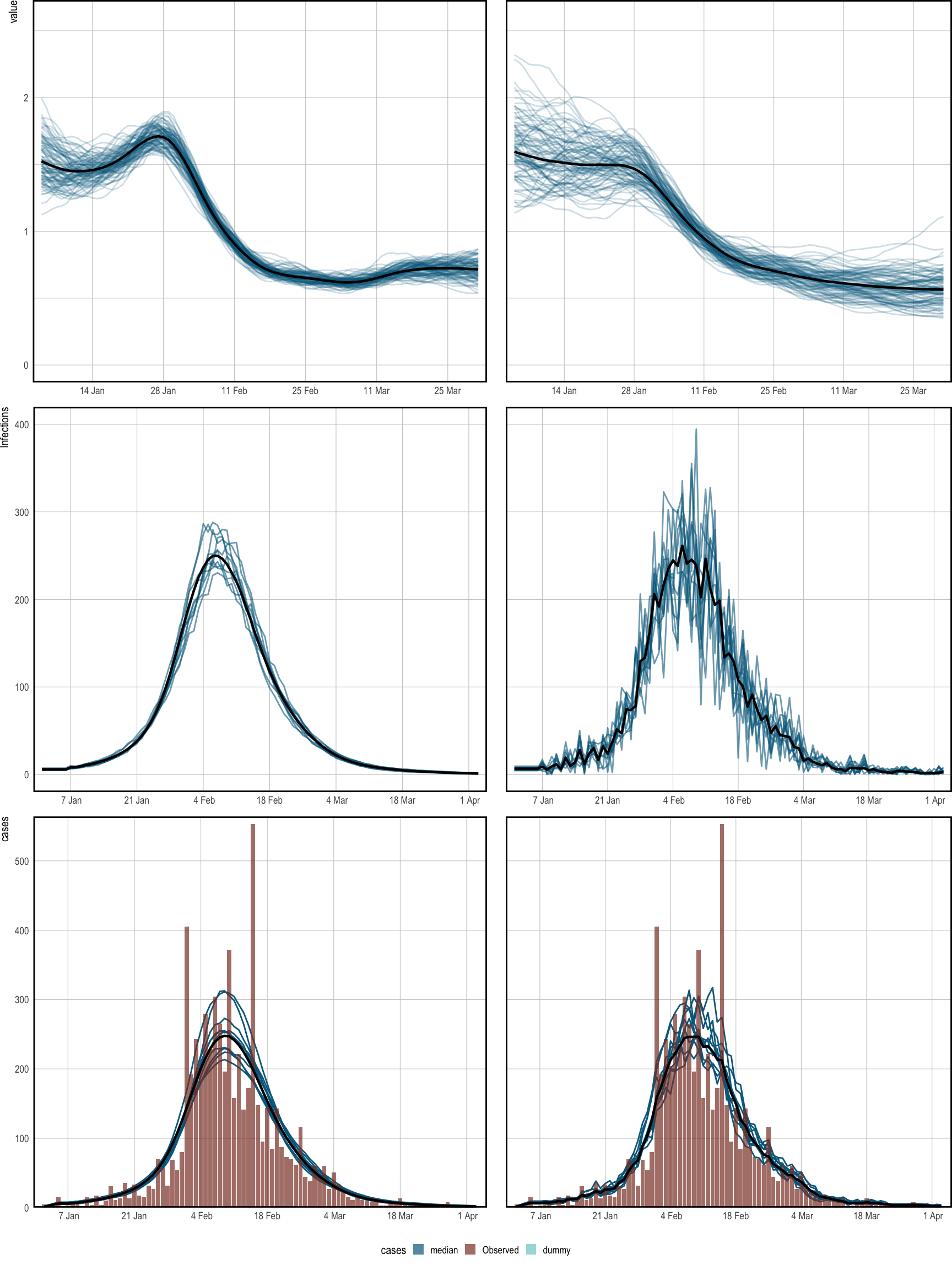
Spaghetti plots showing the median (black) and sample paths (blue) from the posterior distribution. The **left** corresponds to the basic model, and the **right** panel is for the extended version. **Top**: inferred time-varying reproduction numbers, which have been smoothed over 7 days for illustration. **Middle**: Inferred latent infections. **Bottom**: observed cases, and cases simulated from the posterior. These align closely, and so do not flag problems with the model fit.