Model Reproduction Rates

epirt defines a model for reproduction rates. For more details on the model assumptions, please read the model description vignette.

epirt(
  formula,
  link = "log",
  center = FALSE,
  prior = rstanarm::normal(scale = 0.5),
  prior_intercept = rstanarm::normal(scale = 0.5),
  prior_covariance = rstanarm::decov(scale = 0.5),
  ...
)

Arguments

formula	An object of class formula which determines the linear predictor for the reproduction rates. The left hand side must take the form R(group, date), where group and date variables. group must be a factor vector indicating group membership (i.e. country, state, age cohort), and date must be a vector of class Date. This is syntactic sugar for the reproduction number in the given group at the given date.
link	The link function. This must be either "identity", "log", or a call to scaled_logit.
center	If TRUE then the covariates for the regression are centered to have mean zero. All of the priors are then interpreted as prior on the centered covariates. Defaults to FALSE.
prior	Same as in stan_glm. In addition to the rstanarm provided priors, a shifted_gamma can be used. Note: If autoscale=TRUE in the call to the prior distribution then automatic rescaling of the prior may take place.
prior_intercept	Same as in stan_glm. Prior for the regression intercept (if it exists).
prior_covariance	Same as in stan_glmer. Only used if the formula argument specifies random effects.
...	Additional arguments for model.frame

Value

An object of class epirt.

Details

epirt has a formula argument which defines the linear predictor, an argument link defining the link function, and additional arguments to specify priors on parameters making up the linear predictor.

A general R formula gives a symbolic description of a model. It takes the form y ~ model, where y is the response and model is a collection of terms separated by the + operator. model fully defines a linear predictor used to predict y. In this case, the “response” being modeled are reproduction numbers which are unobserved. epirt therefore requires that the left hand side of the formula takes the form R(group, date), where group and date refer to variables representing the region and date respectively. The right hand side can consist of fixed effects, random effects, and autocorrelation terms.

Examples

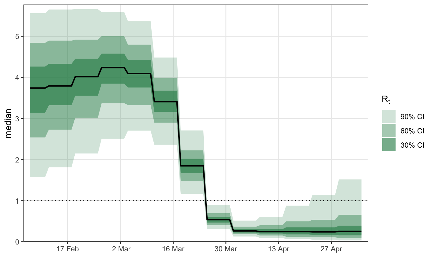
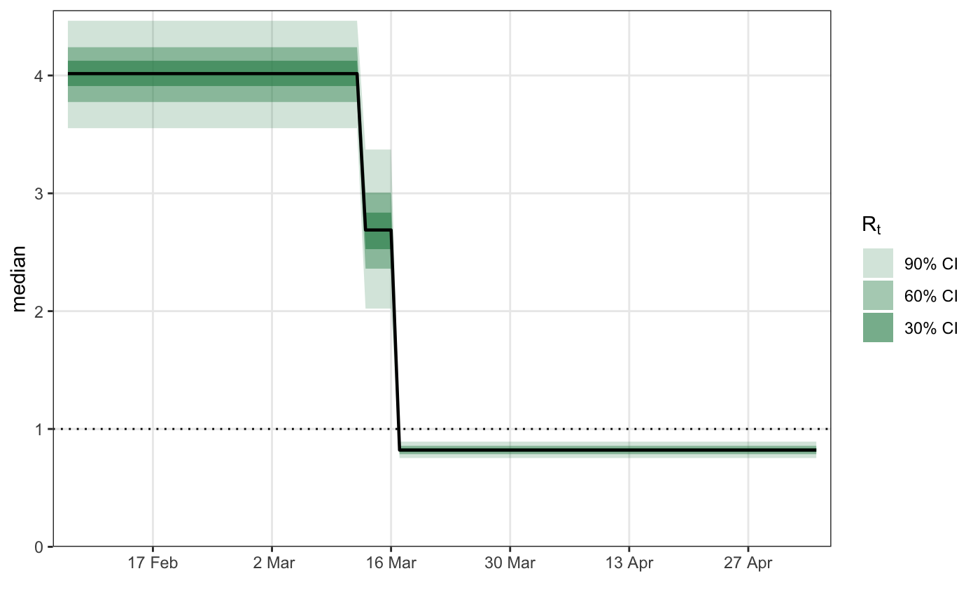
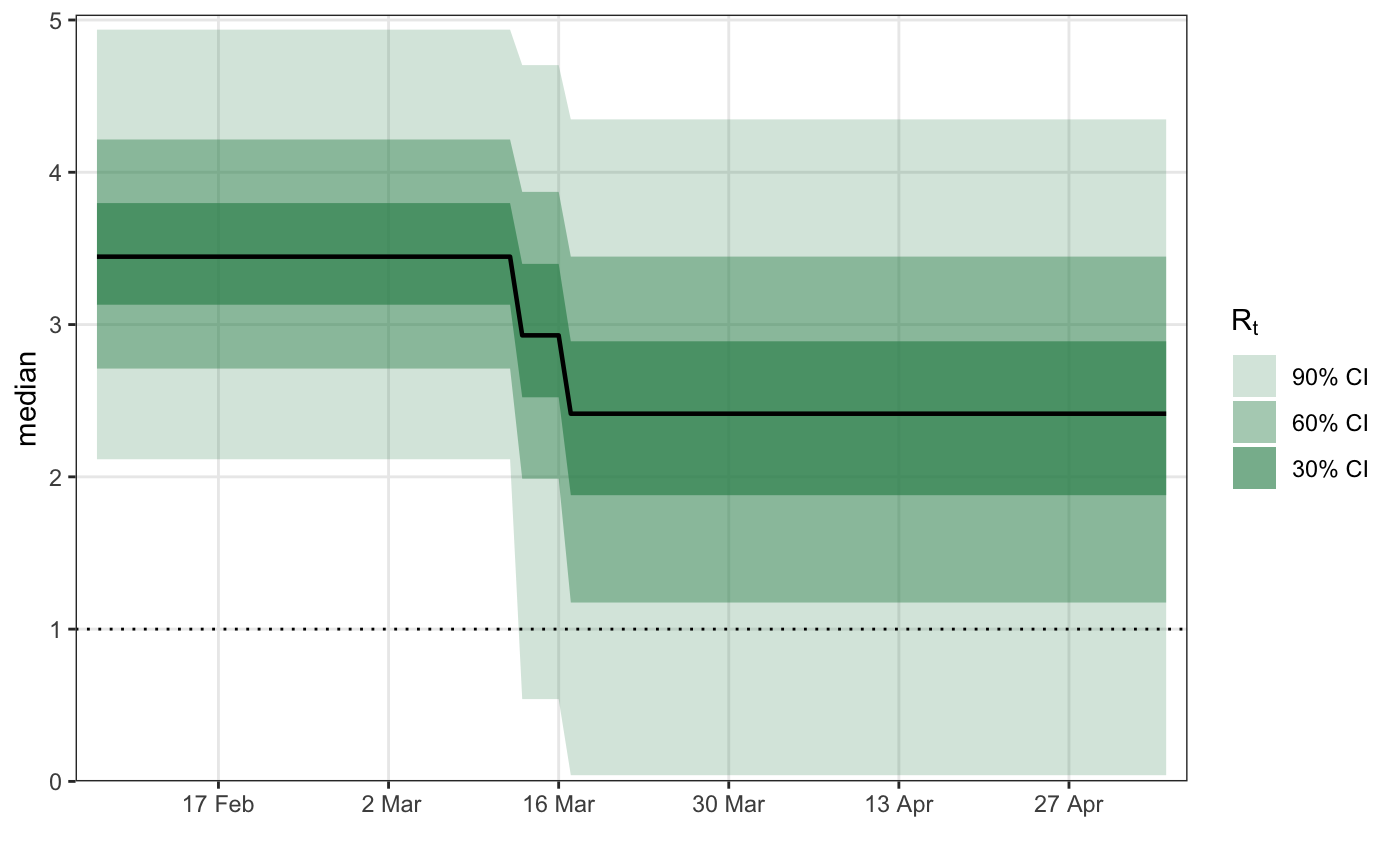
# \donttest{
library(epidemia)
library(ggplot2)
data("EuropeCovid")
options(mc.cores = parallel::detectCores())

data <- EuropeCovid$data
data$week <- lubridate::week(data$date)

# collect arguments for epim
args <- list(
  inf = epiinf(gen = EuropeCovid$si),
  obs = epiobs(deaths ~ 1, i2o = EuropeCovid$inf2death, link = scaled_logit(0.02)),
  data = data,
  algorithm = "fullrank", # For speed - should generally use "sampling"
  iter = 2e4,
  group_subset = "France",
  seed = 12345,
  refresh = 0
)

# a simple random walk model for R
args$rt <- epirt(
  formula = R(country, date) ~ rw(time = week),
  link = scaled_logit(7)
)

fm1 <- do.call(epim, args)
#> Warning: Pareto k diagnostic value is 0.79. Resampling is unreliable. Increasing the number of draws or decreasing tol_rel_obj may help.
plot_rt(fm1) + theme_bw()

# Modeling effects of NPIs
args$rt <- epirt(
  formula = R(country, date) ~ 1 + lockdown + public_events,
  link = scaled_logit(7)
)

fm2 <- do.call(epim, args)
#> Warning: Pareto k diagnostic value is 1.62. Resampling is disabled. Decreasing tol_rel_obj may help if variational algorithm has terminated prematurely. Otherwise consider using sampling instead.
plot_rt(fm2) + theme_bw()


# shifted gamma prior for NPI effects
args$rt <- epirt(
  formula = R(country, date) ~ 1 + lockdown + public_events,
  link = scaled_logit(7),
  prior = shifted_gamma(shape = 1/2, scale = 1, shift = log(1.05)/2)
)

# How does the implied prior look?
args$prior_PD <- TRUE
fm3 <- do.call(epim, args)
#> Warning: Pareto k diagnostic value is 0.71. Resampling is unreliable. Increasing the number of draws or decreasing tol_rel_obj may help.
plot_rt(fm3) + theme_bw()
# }