
Case Study 4 - GPU Computing User
Last updated on 2026-07-30 | Edit this page
Estimated time: 60 minutes
Overview
Questions
- How can prior training run data and local benchmark timings be used to estimate the carbon footprint of a new model before committing to a full training run?
- What is the carbon cost of training a deep learning model naively compared to using optimisations such as transfer learning, mixed precision, and early stopping?
- How do ML-specific choices — optimiser, batch size, model architecture — affect both GPU memory requirements, utilisation efficiency, and carbon emissions?
- What are the trade-offs between running training jobs on cloud GPU infrastructure versus a local workstation?
Objectives
- Estimate the carbon footprint of a deep learning training run using proxy data from a previous run and local benchmark timings.
- Identify sources of wasted computation in a naive model training workflow and prioritise opportunities for reduction.
- Evaluate the carbon impact of ML optimisations including transfer learning, mixed-precision training, early stopping, and model architecture choices.
- Compare the carbon cost and practical trade-offs of local versus cloud GPU training.
Scenario

His primary responsibilities are:
- The deployment of cutting edge deep learning models
- Periodic maintenance of models to add features and prevent model drift
- The curation and storing of large datasets
To do his work, Miguel often trains and fine-tunes models on his local GPU-equipped workstation when the job is small enough, and offloads larger jobs to dedicated cloud GPU compute providers.
Miguel is tasked with deploying a new model to the cloud, based on the architecture of an existing model he deployed last year. The existing model was trained with vast quantities of real animal images, and is already quite competent at feline-based image processing. It performed simple detection of cats in images, but the new model must produce bounding boxes. The previous training script was very crude, and simply passed the entire dataset through the model in batches of 256, for exactly 100 epochs of stochastic gradient descent (SGD), with no regularisation.
Based on his experience preparing the previous model, he knows that his workstation’s GPU will not have enough memory to train the similarly-sized derived model with a reasonable batch size in its current form. Like last time, he will aim to offload the training of the model to a cloud GPU compute provider, however local development and fine-tuning will still be possible using a very small batch size.
Before committing cloud compute resources, Miguel wants to estimate the carbon cost of his planned training run and explore ways to reduce it — both to keep emissions low and to avoid an expensive wasted run if something goes wrong.
Collecting Information
Data Exploration (20 minutes)
Miguel’s work consists of developing and fine-tuning the model on his local workstation, followed by training and deploying the model on cloud infrastructure. How might Miguel estimate the associated carbon emissions? What data will be required, and how might he find such data?
There are various methods Miguel can build a picture of carbon emissions with, including real-time measurement, prediction tools and extrapolaring from known data.
- Realtime measurement can be performed locally using either a physical meter measuring power usage directly from the mains socket, or by wrapping code with power monitoring software packages such as CodeCarbon. Realtime measurement of cloud jobs may also be possible, since many cloud providers offer infrastructure for querying live energy usage of running jobs.
- Carbon data from training the previous model may be used as surrogate data for the new model, given their near-identical architecture. If carbon data for the previous run was not recorded, then predictive tools can be used to estimate it. For example, the Green Algorithms Calculator may be used to estimate carbon data of a previous job given its runtime, server location and compute requirements.
Analysis
Estimating Emissions (20 minutes)
Miguel uses 2 methods to get estimates up-front of the carbon footprint of a full training run.
Local Development and Testing
Miguel is unable to train the model at target batch size of 256 on his workstation, but information from a smaller run might still be useful for estimating the carbon emissions of the larger run. He decides to use CodeCarbon to measure the power consumption of his CPU and GPU for a single training epoch, using 1% of the training data, with a batch size of 32.
CodeCarbon reports an energy usage of 430 Wh over 5 hours during this test run.
Use this value to estimate the energy required and carbon emissions for a full training run.
Previous Training Runs
Given the similarity of the new model to the old one, data obtained during the training run of the previous model may be used as surrogate data for estimating the carbon usage of the newer model. He remembers that the previous job ran for approximately 72 hours, and used the Azure (Southern UK) datacentre with the following hardware:
- 64 GB of available host RAM
- Eight virtual cores of an Intel Xeon Platinum 8260 CPU
- One whole NVIDIA Tesla V100 GPU
Use the Green Algorithms
Calculator to estimate the energy usage and carbon footprint of
training the new model using information obtained from training the
similar previous model. For this exercise, select data version
v3.0 in the top right of the calculator page.
Miguel’s results for the two estimate methods are as follows.
Local Development and Testing
Since the test run used 1% of the training data, scaling the measured energy up to the full dataset gives:
\[ 430 \text{ Wh} \times 100 = 43{,}000 \text{ Wh} = \textbf{43 kWh} \]
Using the 2025 UK average carbon intensity of 126 g/kWh this gives a total of 5.4 kgCO2e.
Previous Training Runs
Plugging in the runtime, hardware and location of the job into the calculator, it estimates that 30.55 kWh of energy was required to train the model, with a carbon footprint of 7.06 kgCO2e.
Comparing
The two methods give estimates of 43 kWh (5.4 kgCO₂e)and 30.55 kWh (7.06 kgCO₂e), which are in rough agreement given the approximations involved. Some differences:
Energy estimates (43 vs 30.55 kWh): The local benchmark is likely an overestimate of the cloud run’s energy consumption. The test run uses a smaller batch size and local consumer-grade hardware, both of which tend to be less energy-efficient than the cloud data centre’s server-grade GPUs. The Green Algorithms Calculator estimate is based on component TDP values rather than real utilisation, which tends to overestimate, partially offsetting this.
Carbon intensity (5.4 vs 7.06 kgCO₂e): The local estimate uses the UK average grid intensity (126 gCO₂/kWh), while the Green Algorithms Calculator uses a location- and provider-specific value for Azure Southern UK. The latter also applies a PUE factor to account for data centre cooling and infrastructure overhead — an overhead not captured by CodeCarbon on the local workstation.
Strengths and weaknesses:
| Local benchmark (CodeCarbon) | Surrogate data (Green Algorithms Calculator) | |
|---|---|---|
| Energy measurement | Directly measured (actual power draw) | Estimated from TDP (may over/underestimate) |
| Hardware match | Different from cloud run | More representative of planned training |
| Carbon intensity | UK average | Provider- and location-specific |
| Overheads accounted for | No | Yes |
| Overall | Good for bounding the estimate; captures real utilisation on local hardware | More representative of the actual cloud run |
Additional data that would improve both estimates: real-time carbon intensity at the time and location of the run; GPU utilisation metrics from the cloud provider; the data centre’s actual PUE; and actual energy billing data from the cloud provider if available, as some providers now expose this directly.
Given the above, the surrogate data estimate of (7.06 kgCO₂e) is the more representative figure for the planned cloud training run, as long as it’s run in the same location, and we’ll use it as the baseline going forward.
Taking Action
Reducing emissions from model training (20 minutes)
Miguel’s estimates suggest that a naive training run — repeating the same approach used for the previous model — would cost approximately 7.06 kgCO₂e. In your groups, discuss what strategies Miguel could use to reduce this. Consider:
- Are there any aspects of the naive training approach that represent unnecessary computation?
- What ML-specific techniques could reduce the number of training steps required?
- What are the trade-offs between training on a cloud GPU versus a local workstation, from both a carbon and a practical perspective?
From his observations, Miguel formulates a plan. It is clear to him that it is entirely unnecessary to train a new model from scratch, given the prior model is already quite competent at processing cats. The existing model can readily be adapted by appending a new head for cat bounding-boxes, and transfer learning techniques can be utilised to further fine-tune the model to a reasonable accuracy.
Miguel begins to quantify the computational resources required to train the revised model. With bytes per value \(b = 4\), number of trainable parameters \(P ≈ 26,000,000\), batch size \(M = 256\) and number of activation state variables for all layers \(N ≈ 11,000,000\):
| Memory Type | Formula | Size (bytes) |
|---|---|---|
| Parameters | \(P \cdot b\) | \(104,000,000\) |
| Gradients | \(P \cdot b\) | \(104,000,000\) |
| Optimiser State | \(P \cdot k \cdot b\) | \(0\) |
| Activation State | \(M \cdot N \cdot b\) | \(11,264,000,000\) |
An extra \(20\% ≈ 2,294,400,000\) bytes overhead for internal ML framework usage is also included, totalling approximately \(12.8\) GB. In general, there is an optimiser memory factor \(k\), but plain SGD has no internal state, hence \(k = 0\) for now. With this estimation framework, he is able to know upfront roughly how much GPU memory the job will require, as a function of batch and layer size. Whilst the SGD optimiser reduces the memory required to train the model, via \(k = 0\) above, the prospect of earlier convergence using an alternative optimiser with \(k > 0\) may make the memory increase overall worthwhile.
He begins experimenting, appending the new bounding-box head and starting training, keeping the trainable parameters in the body fixed, and gradually relaxing them as training progresses. He modifies the training script to back up training state after each epoch, to avoid starting again on software crash or hardware failure. He is able to greatly increase the convergence rate with a moderate increase in required memory (\(k = 2\) in the memory equations) using the more sophisticated Adam optimiser, and further improves it by adding a learning rate decay. With the convergence rate noticeably increased, he adds logic to terminate early once the model’s loss function converges. The 32-bit floating-point numbers for activation state and gradients are switched to 16-bit, increasing operator speed and halving the memory required for both.
Miguel takes another look at the model’s architecture, and notes that it is very large for its stated purpose, with many channels per convolutional layer, and very wide fully connected layers in the head. He wonders if the model can be pruned to enable training on his workstation, instead of relying on the cloud provider. Noting again that the model is very large for its stated purpose, Miguel adds L1 (Lasso) regularisation to reduce redundant activation, allowing many (now-unused) activation units to be removed from the model entirely, resulting in a \(20\%\) memory saving.
With the model now small enough to run efficiently on his workstation, Miguel runs a short test-run to check that all is well before the main training run. He notes that even on his relatively small GPU, the model is not utilising his GPU entirely. Since a partially-occupied GPU is disproportionally less efficient than an occupied one, he estimates the memory requirements of this revised model, with the aim of maximising batch size to better-utilise the GPU. With new values \(b_{16} = 2\), \(b_{32} = 4\), \(P ≈ 20,800,000\), \(k = 2\), \(M = 256\) and \(N ≈ 8,800,000\):
| Memory Type | Formula | Size (bytes) |
|---|---|---|
| Parameters | \(P \cdot b_{32}\) | \(83,200,000\) |
| Gradients | \(P \cdot b_{16}\) | \(41,600,000\) |
| Optimiser State | \(P \cdot k \cdot b_{32}\) | \(166,400,000\) |
| Activation State | \(M \cdot N \cdot b_{16}\) | \(4,505,600,000\) |
and extra \(20\% ≈ 959,360,000\) bytes overhead, totalling approximately \(5.4\) GB only. Indeed, Miguel finds he can increase batch size even up to \(M = 728\) before the \(16\) GB of memory from the previous job comes close to full, potentially tripling job speed on the same hardware.
These experiments highlight the dramatic computational efficiency increases that can be achieved with careful optimisation of the job. Naive implementation of training and inference can have a considerably higher carbon footprint, requiring larger GPUs and longer run times, while carefully optimised workflows can be run very quickly and be small enough to run on local hardware.
It can often be the case that running AI workflows on cloud providers has a smaller carbon footprint than running on local hardware. The energy efficiency measures of datacentres make operational carbon relatively lower than smaller dedicated hardware setups, and embedded carbon can be lower using existing datacentre hardware, compared to buying and decommissioning in-house hardware. The flipside is that one looses the ability to choose when a job is executed, meaning demand shifting to off-peak times is no longer an option. In either case, Miguel’s optimisations have had a huge effect on the model’s carbon footprint, and have afforded him the choice of using either, depending on the circumstances.
Outcomes
After completing his optimisations Miguel runs some more tests and finds an 83% reduction in computation time running on the same hardware. He uses this factor to estimate the carbon savings of training his models in the cloud.
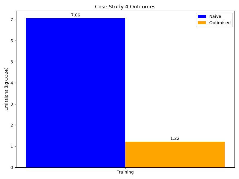
The table below summarises the key changes Miguel made:
| Naive approach | Optimised approach | |
|---|---|---|
| Training strategy | From scratch (100 epochs, full dataset) | Transfer learning + early stopping |
| Optimiser | SGD | Adam with learning rate decay |
| Numerical precision | FP32 throughout | Mixed precision (FP32/FP16) |
| Estimated power consumption (cloud) | 30.55 kWh | 5.3 kWh |
| Carbon footprint (kgCO₂e) | 7.06 | 1.22 |
- Prior training run data and local benchmark timings can be combined to estimate emissions before committing to an expensive full training run.
- Naive ML training workflows often contain significant avoidable computation — training from scratch when transfer learning is possible is a common and costly example.
- ML-specific optimisations (transfer learning, early stopping, mixed precision, model pruning) can reduce both training time and GPU memory requirements, often by an order of magnitude.
- Maximising GPU utilisation through right-sized batch sizes improves energy efficiency; a partially-occupied GPU is disproportionately less efficient than a fully-occupied one.
- Cloud training offers lower operational carbon through data centre efficiency but removes the option to demand-shift; local training restores that flexibility at the cost of higher embodied emissions per unit of compute.