Analysing data with NumPy

Overview

Teaching: 15 min
Exercises: 15 min

Questions

• How can I import and analyse tabular data files in Python?

Objectives

• Read tabular data from a file into a program.

• Select individual values and subsections from data.

• Perform operations on arrays of data.

Loading data into Python

In order to load our inflammation data, we need to access (import in Python terminology) a library called NumPy. In general you should use this library if you want to do fancy things with numbers, especially if you have matrices or arrays. We can import NumPy using:

import numpy

Importing a library is like getting a piece of lab equipment out of a storage locker and setting it up on the bench. Libraries provide additional functionality to the basic Python package, much like a new piece of equipment adds functionality to a lab space. Just like in the lab, importing too many libraries can sometimes complicate and slow down your programs - so we only import what we need for each program. Once we’ve imported the library, we can ask the library to read our data file for us:

numpy.loadtxt(fname='inflammation-01.csv', delimiter=',')

array([[ 0.,  0.,  1., ...,  3.,  0.,  0.],
       [ 0.,  1.,  2., ...,  1.,  0.,  1.],
       [ 0.,  1.,  1., ...,  2.,  1.,  1.],
       ...,
       [ 0.,  1.,  1., ...,  1.,  1.,  1.],
       [ 0.,  0.,  0., ...,  0.,  2.,  0.],
       [ 0.,  0.,  1., ...,  1.,  1.,  0.]])

The expression numpy.loadtxt(...) is a function call that asks Python to run the function loadtxt which belongs to the numpy library. This dotted notation is used everywhere in Python: the thing that appears before the dot contains the thing that appears after.

As an example, John Smith is the John that belongs to the Smith family. We could use the dot notation to write his name smith.john, just as loadtxt is a function that belongs to the numpy library.

numpy.loadtxt has two parameters: the name of the file we want to read and the delimiter that separates values on a line. These both need to be character strings (or strings for short), so we put them in quotes.

Since we haven’t told it to do anything else with the function’s output, the notebook displays it. In this case, that output is the data we just loaded. By default, only a few rows and columns are shown (with ... to omit elements when displaying big arrays). To save space, Python displays numbers as 1. instead of 1.0 when there’s nothing interesting after the decimal point.

Our call to numpy.loadtxt read our file but didn’t save the data in memory. To do that, we need to assign the array to a variable. Just as we can assign a single value to a variable, we can also assign an array of values to a variable using the same syntax. Let’s re-run numpy.loadtxt and save the returned data:

data = numpy.loadtxt(fname='inflammation-01.csv', delimiter=',')

This statement doesn’t produce any output because we’ve assigned the output to the variable data. If we want to check that the data have been loaded, we can print the variable’s value:

print(data)

[[ 0.  0.  1. ...,  3.  0.  0.]
 [ 0.  1.  2. ...,  1.  0.  1.]
 [ 0.  1.  1. ...,  2.  1.  1.]
 ...,
 [ 0.  1.  1. ...,  1.  1.  1.]
 [ 0.  0.  0. ...,  0.  2.  0.]
 [ 0.  0.  1. ...,  1.  1.  0.]]

Now that the data are in memory, we can manipulate them. First, let’s ask what type of thing data refers to:

print(type(data))

<class 'numpy.ndarray'>

The output tells us that data currently refers to an N-dimensional array, the functionality for which is provided by the NumPy library. These data correspond to arthritis patients’ inflammation. The rows are the individual patients, and the columns are their daily inflammation measurements.

Data Type

A Numpy array contains one or more elements of the same type. The type function will only tell you that a variable is a NumPy array but won’t tell you the type of thing inside the array. We can find out the type of the data contained in the NumPy array.

print(data.dtype)

dtype('float64')

This tells us that the NumPy array’s elements are floating-point numbers.

With the following command, we can see the array’s shape:

print(data.shape)

(60, 40)

The output tells us that the data array variable contains 60 rows and 40 columns. When we created the variable data to store our arthritis data, we didn’t just create the array; we also created information about the array, called members or attributes. This extra information describes data in the same way an adjective describes a noun. data.shape is an attribute of data which describes the dimensions of data. We use the same dotted notation for the attributes of variables that we use for the functions in libraries because they have the same part-and-whole relationship.

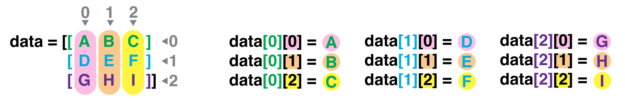
If we want to get a single number from the array, we must provide an index in square brackets after the variable name, just as we do in math when referring to an element of a matrix. Our inflammation data has two dimensions, so we will need to use two indices to refer to one specific value:

print('first value in data:', data[0, 0])

first value in data: 0.0

print('middle value in data:', data[30, 20])

middle value in data: 13.0

The expression data[30, 20] accesses the element at row 30, column 20. While this expression may not surprise you, data[0, 0] might. Programming languages like Fortran, MATLAB and R start counting at 1 because that’s what human beings have done for thousands of years. Languages in the C family (including C++, Java, Perl, and Python) count from 0 because it represents an offset from the first value in the array (the second value is offset by one index from the first value). This is closer to the way that computers represent arrays (if you are interested in the historical reasons behind counting indices from zero, you can read Mike Hoye’s blog post). As a result, if we have an M×N array in Python, its indices go from 0 to M-1 on the first axis and 0 to N-1 on the second. It takes a bit of getting used to, but one way to remember the rule is that the index is how many steps we have to take from the start to get the item we want.

In the Corner

What may also surprise you is that when Python displays an array, it shows the element with index [0, 0] in the upper left corner rather than the lower left. This is consistent with the way mathematicians draw matrices but different from the Cartesian coordinates. The indices are (row, column) instead of (column, row) for the same reason, which can be confusing when plotting data.

Slicing data

An index like [30, 20] selects a single element of an array, but we can select whole sections as well. For example, we can select the first ten days (columns) of values for the first four patients (rows) like this:

print(data[0:4, 0:10])

[[ 0.  0.  1.  3.  1.  2.  4.  7.  8.  3.]
 [ 0.  1.  2.  1.  2.  1.  3.  2.  2.  6.]
 [ 0.  1.  1.  3.  3.  2.  6.  2.  5.  9.]
 [ 0.  0.  2.  0.  4.  2.  2.  1.  6.  7.]]

The slice 0:4 means, “Start at index 0 and go up to, but not including, index 4.”Again, the up-to-but-not-including takes a bit of getting used to, but the rule is that the difference between the upper and lower bounds is the number of values in the slice.

We don’t have to start slices at 0:

print(data[5:10, 0:10])

[[ 0.  0.  1.  2.  2.  4.  2.  1.  6.  4.]
 [ 0.  0.  2.  2.  4.  2.  2.  5.  5.  8.]
 [ 0.  0.  1.  2.  3.  1.  2.  3.  5.  3.]
 [ 0.  0.  0.  3.  1.  5.  6.  5.  5.  8.]
 [ 0.  1.  1.  2.  1.  3.  5.  3.  5.  8.]]

We also don’t have to include the upper and lower bound on the slice. If we don’t include the lower bound, Python uses 0 by default; if we don’t include the upper, the slice runs to the end of the axis, and if we don’t include either (i.e., if we just use ‘:’ on its own), the slice includes everything:

small = data[:3, 36:]
print('small is:')
print(small)

The above example selects rows 0 through 2 and columns 36 through to the end of the array.

small is:
[[ 2.  3.  0.  0.]
 [ 1.  1.  0.  1.]
 [ 2.  2.  1.  1.]]

Arrays also know how to perform common mathematical operations on their values. The simplest operations with data are arithmetic: addition, subtraction, multiplication, and division. When you do such operations on arrays, the operation is done element-by-element. Thus:

doubledata = data * 2.0

will create a new array doubledata each element of which is twice the value of the corresponding element in data:

print('original:')
print(data[:3, 36:])
print('doubledata:')
print(doubledata[:3, 36:])

original:
[[ 2.  3.  0.  0.]
 [ 1.  1.  0.  1.]
 [ 2.  2.  1.  1.]]
doubledata:
[[ 4.  6.  0.  0.]
 [ 2.  2.  0.  2.]
 [ 4.  4.  2.  2.]]

If, instead of taking an array and doing arithmetic with a single value (as above), you did the arithmetic operation with another array of the same shape, the operation will be done on corresponding elements of the two arrays. Thus:

tripledata = doubledata + data

will give you an array where tripledata[0,0] will equal doubledata[0,0] plus data[0,0], and so on for all other elements of the arrays.

print('tripledata:')
print(tripledata[:3, 36:])

tripledata:
[[ 6.  9.  0.  0.]
 [ 3.  3.  0.  3.]
 [ 6.  6.  3.  3.]]

Often, we want to do more than add, subtract, multiply, and divide array elements. NumPy knows how to do more complex operations, too. If we want to find the average inflammation for all patients on all days, for example, we can ask NumPy to compute data’s mean value:

print(numpy.mean(data))

6.14875

mean is a function that takes an array as an argument.

Not All Functions Have Input

Generally, a function uses inputs to produce outputs. However, some functions produce outputs without needing any input. For example, checking the current time doesn’t require any input.

import time
print(time.ctime())

'Sat Mar 26 13:07:33 2016'

For functions that don’t take in any arguments, we still need parentheses (()) to tell Python to go and do something for us.

NumPy has lots of useful functions that take an array as input. Let’s use three of those functions to get some descriptive values about the dataset. We’ll also use multiple assignment, a convenient Python feature that will enable us to do this all in one line.

maxval, minval, stdval = numpy.max(data), numpy.min(data), numpy.std(data)

print('maximum inflammation:', maxval)
print('minimum inflammation:', minval)
print('standard deviation:', stdval)

Here we’ve assigned the return value from numpy.max(data) to the variable maxval, the value from numpy.min(data) to minval, and so on.

maximum inflammation: 20.0
minimum inflammation: 0.0
standard deviation: 4.61383319712

Mystery Functions in IPython

How did we know what functions NumPy has and how to use them? If you are working in the IPython/Jupyter Notebook, there is an easy way to find out. If you type the name of something followed by a dot, then you can use tab completion (e.g. type numpy. and then press tab) to see a list of all functions and attributes that you can use. After selecting one, you can also add a question mark (e.g. numpy.cumprod?), and IPython will return an explanation of the method! This is the same as doing help(numpy.cumprod).

When analyzing data, though, we often want to look at variations in statistical values, such as the maximum inflammation per patient or the average inflammation per day. One way to do this is to create a new temporary array of the data we want, then ask it to do the calculation:

patient_0 = data[0, :] # 0 on the first axis (rows), everything on the second (columns)
print('maximum inflammation for patient 0:', patient_0.max())

maximum inflammation for patient 0: 18.0

Everything in a line of code following the ‘#’ symbol is a comment that is ignored by Python. Comments allow programmers to leave explanatory notes for other programmers or their future selves.

We don’t actually need to store the row in a variable of its own. Instead, we can combine the selection and the function call:

print('maximum inflammation for patient 2:', numpy.max(data[2, :]))

maximum inflammation for patient 2: 19.0

What if we need the maximum inflammation for each patient over all days (as in the next diagram on the left) or the average for each day (as in the diagram on the right)? As the diagram below shows, we want to perform the operation across an axis:

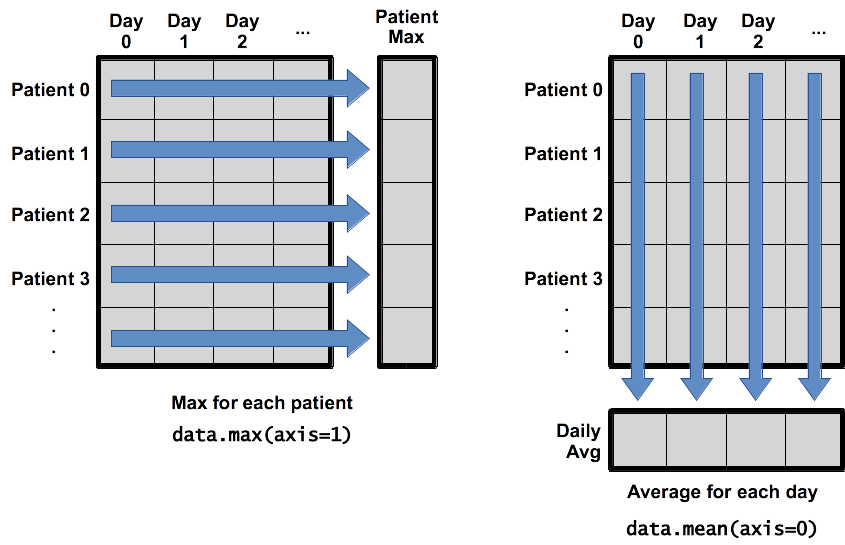
To support this functionality, most array functions allow us to specify the axis we want to work on. If we ask for the average across axis 0 (rows in our 2D example), we get:

print(numpy.mean(data, axis=0))

[  0.           0.45         1.11666667   1.75         2.43333333   3.15
   3.8          3.88333333   5.23333333   5.51666667   5.95         5.9
   8.35         7.73333333   8.36666667   9.5          9.58333333
  10.63333333  11.56666667  12.35        13.25        11.96666667
  11.03333333  10.16666667  10.           8.66666667   9.15         7.25
   7.33333333   6.58333333   6.06666667   5.95         5.11666667   3.6
   3.3          3.56666667   2.48333333   1.5          1.13333333
   0.56666667]

As a quick check, we can ask this array what its shape is:

print(numpy.mean(data, axis=0).shape)

(40,)

The expression (40,) tells us we have an N×1 vector, so this is the average inflammation per day for all patients. If we average across axis 1 (columns in our 2D example), we get:

print(numpy.mean(data, axis=1))

[ 5.45   5.425  6.1    5.9    5.55   6.225  5.975  6.65   6.625  6.525
  6.775  5.8    6.225  5.75   5.225  6.3    6.55   5.7    5.85   6.55
  5.775  5.825  6.175  6.1    5.8    6.425  6.05   6.025  6.175  6.55
  6.175  6.35   6.725  6.125  7.075  5.725  5.925  6.15   6.075  5.75
  5.975  5.725  6.3    5.9    6.75   5.925  7.225  6.15   5.95   6.275  5.7
  6.1    6.825  5.975  6.725  5.7    6.25   6.4    7.05   5.9  ]

which is the average inflammation per patient across all days.

Encapsulation

Fill in the blanks to create a function that takes a single filename, containing comma separated values, as an argument, loads the data in the file named by the argument, and returns the minimum value in that data.

import numpy

def min_in_data(____):
    data = ____
    return ____

Solution

import numpy

def min_in_data(filename):
    data = numpy.loadtxt(fname=filename, delimiter=',')
    return data.min()

Stacking Arrays

Arrays can be concatenated and stacked on top of one another, using NumPy’s vstack and hstack functions for vertical and horizontal stacking, respectively.

import numpy

A = numpy.array([[1,2,3], [4,5,6], [7, 8, 9]])
print('A = ')
print(A)

B = numpy.hstack([A, A])
print('B = ')
print(B)

C = numpy.vstack([A, A])
print('C = ')
print(C)

A =
[[1 2 3]
 [4 5 6]
 [7 8 9]]
B =
[[1 2 3 1 2 3]
 [4 5 6 4 5 6]
 [7 8 9 7 8 9]]
C =
[[1 2 3]
 [4 5 6]
 [7 8 9]
 [1 2 3]
 [4 5 6]
 [7 8 9]]

Write some additional code that slices the first and last columns of A, and stacks them into a 3x2 array. Make sure to print the results to verify your solution.

Solution

A ‘gotcha’ with array indexing is that singleton dimensions are dropped by default. That means A[:, 0] is a one dimensional array, which won’t stack as desired. To preserve singleton dimensions, the index itself can be a slice or array. For example, A[:, :1] returns a two dimensional array with one singleton dimension (i.e. a column vector).

D = numpy.hstack((A[:, :1], A[:, -1:]))
print('D = ')
print(D)

D =
[[1 3]
 [4 6]
 [7 9]]

Solution

An alternative way to achieve the same result is to use Numpy’s delete function to remove the second column of A.

D = numpy.delete(A, 1, 1)
print('D = ')
print(D)

D =
[[1 3]
 [4 6]
 [7 9]]

Change In Inflammation

This patient data is longitudinal in the sense that each row represents a series of observations relating to one individual. This means that the change in inflammation over time is a meaningful concept.

The numpy.diff() function takes a NumPy array and returns the differences between two successive values along a specified axis. For example, a NumPy array that looks like this:

npdiff = numpy.array([ 0,  2,  5,  9, 14])

Calling numpy.diff(npdiff) would do the following calculations and put the answers in another array.

[ 2 - 0, 5 - 2, 9 - 5, 14 - 9 ]

numpy.diff(npdiff)

array([2, 3, 4, 5])

Which axis would it make sense to use this function along?

Solution

Since the row axis (0) is patients, it does not make sense to get the difference between two arbitrary patients. The column axis (1) is in days, so the difference is the change in inflammation – a meaningful concept.

numpy.diff(data, axis=1)

If the shape of an individual data file is (60, 40) (60 rows and 40 columns), what would the shape of the array be after you run the diff() function and why?

Solution

The shape will be (60, 39) because there is one fewer difference between columns than there are columns in the data.

How would you find the largest change in inflammation for each patient? Does it matter if the change in inflammation is an increase or a decrease?

Solution

By using the numpy.max() function after you apply the numpy.diff() function, you will get the largest difference between days.

numpy.max(numpy.diff(data, axis=1), axis=1)

array([  7.,  12.,  11.,  10.,  11.,  13.,  10.,   8.,  10.,  10.,   7.,
         7.,  13.,   7.,  10.,  10.,   8.,  10.,   9.,  10.,  13.,   7.,
        12.,   9.,  12.,  11.,  10.,  10.,   7.,  10.,  11.,  10.,   8.,
        11.,  12.,  10.,   9.,  10.,  13.,  10.,   7.,   7.,  10.,  13.,
        12.,   8.,   8.,  10.,  10.,   9.,   8.,  13.,  10.,   7.,  10.,
         8.,  12.,  10.,   7.,  12.])

If inflammation values decrease along an axis, then the difference from one element to the next will be negative. If you are interested in the magnitude of the change and not the direction, the numpy.absolute() function will provide that.

Notice the difference if you get the largest absolute difference between readings.

numpy.max(numpy.absolute(numpy.diff(data, axis=1)), axis=1)

array([ 12.,  14.,  11.,  13.,  11.,  13.,  10.,  12.,  10.,  10.,  10.,
        12.,  13.,  10.,  11.,  10.,  12.,  13.,   9.,  10.,  13.,   9.,
        12.,   9.,  12.,  11.,  10.,  13.,   9.,  13.,  11.,  11.,   8.,
        11.,  12.,  13.,   9.,  10.,  13.,  11.,  11.,  13.,  11.,  13.,
        13.,  10.,   9.,  10.,  10.,   9.,   9.,  13.,  10.,   9.,  10.,
        11.,  13.,  10.,  10.,  12.])

Key Points

• Use the numpy library to work with arrays in Python.

• The expression array.shape gives the shape of an array.

• Use array[x, y] to select a single element from a 2D array.

• Array indices start at 0, not 1.

• All the indexing and slicing that we’ve used on lists and strings also works on arrays.

• Use low:high to specify a slice that includes indices from low to high-1.

• Use numpy.mean(array), numpy.max(array), and numpy.min(array) to calculate simple statistics.

• Use numpy.mean(array, axis=0) or numpy.mean(array, axis=1) to calculate statistics across the specified axis.