Results

Presenting our results in a way that others can understand is important to help us interpret the results.

For this chapter we will need the following R packages: dplyr tidyr lme4 ggplot2 tidyverse broom.mixed

Note: Only install these if you have not already, otherwise go straight to library()

Random intercept model

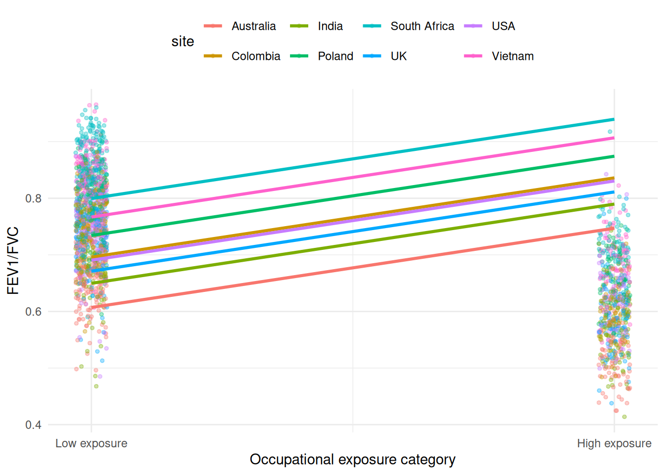
Let’s first assume, we are interested in the overall slope of the relationship between exposure level and lung function (FEV1/FVC).We can check the predicted coefficients.

library(lme4)
clean <- read.table("data/mixed_clean.txt", header=T, sep="\t")
mod_mixed <- lmer(
FEV1_FVC ~ exposure_cat_clean + smoking_status_clean + age + sex_clean + BMI +
(1 | site), data = clean)

#Derive coefficients
model_coefs <- coef(mod_mixed)$site %>%
  as.data.frame() %>%
  rownames_to_column("site") %>%
  rename(
    Intercept = `(Intercept)`,
    Slope = `exposure_cat_cleanlow_exposure`
  ) %>%
  select(site, Intercept, Slope)

model_coefs

          site Intercept     Slope
1    Australia 0.6070478 0.1400147
2     Colombia 0.6960135 0.1400147
3        India 0.6497187 0.1400147
4       Poland 0.7343083 0.1400147
5 South Africa 0.7996435 0.1400147
6           UK 0.6711702 0.1400147
7          USA 0.6905481 0.1400147
8      Vietnam 0.7668158 0.1400147

#Join coefficients to the clean dataset 
clean <- left_join(clean, model_coefs, by = "site")

Graphical representation

#Mutate names
clean <- clean |>
  dplyr::mutate(
    exposure_cat_clean = factor(
      exposure_cat_clean,
      levels = c("low_exposure", "high_exposure")
    ),
    exposure_num = ifelse(exposure_cat_clean == "low_exposure", 0, 1)
  )

coef_df <- model_coefs |>
  tidyr::expand_grid(exposure_num = c(0, 1)) |>
  dplyr::mutate(
    FEV1_FVC_pred = Intercept + Slope * exposure_num
  )


#Plot the results
library(ggplot2)

model_coef_plot <- ggplot(clean, aes(x = exposure_num, y = FEV1_FVC)) +
  # raw points
  geom_point(
    aes(colour = site),
    alpha    = 0.35,
    size     = 1,
    position = position_jitter(width = 0.03, height = 0)
  ) +
  # mixed-model lines
  geom_line(
    data = coef_df,
    aes(x = exposure_num, y = FEV1_FVC_pred, colour = site, group = site),
    size = 1.1
  ) +
  scale_x_continuous(
    name   = "Occupational exposure category",
    breaks = c(0, 1),
    labels = c("Low exposure", "High exposure"),
    expand = expansion(mult = c(0.05, 0.05))
  ) +
  ylab("FEV1/FVC") +
  theme_minimal() +
  theme(legend.position = "top")

model_coef_plot

Caterpillar plots

ran <- broom.mixed::tidy(mod_mixed, effects = "ran_vals") %>%
  filter(term == "(Intercept)") %>%
  mutate(
    site = reorder(level, estimate)  # order by effect size
  )

ggplot(ran, aes(x = estimate, y = site, colour = site)) +
  geom_vline(xintercept = 0, linetype = "dashed", colour = "grey50") +
  geom_point(size = 3) +
  geom_errorbarh(aes(xmin = estimate - 1.96*std.error,
                     xmax = estimate + 1.96*std.error),
                 height = 0.2, size = 0.9) +
  labs(
    title = "Site-Specific Random Intercepts",
        x = "Site deviation from overall intercept",
    y = "Site"
  ) +
  theme_minimal(base_size = 14) +
  theme(
    legend.position = "none",
    plot.title = element_text(face = "bold")
  )

Warning: `geom_errobarh()` was deprecated in ggplot2 4.0.0.
ℹ Please use the `orientation` argument of `geom_errorbar()` instead.

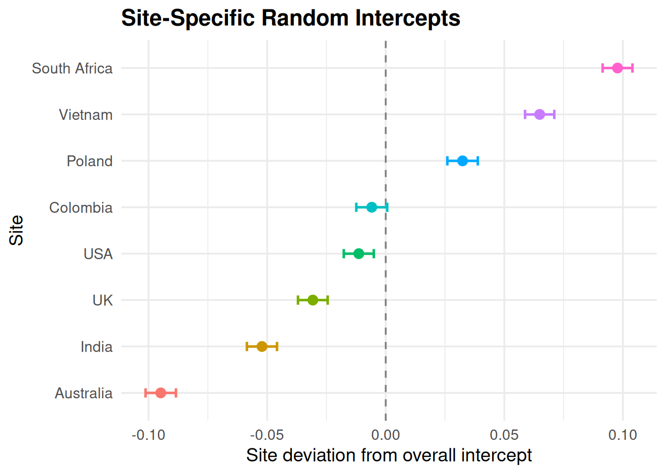
In this plot we can see that the estimated random intercepts from the mixed model, which represent how each site differs from the overall baseline level of FEV1/FVC. Sites with positive values start higher than the mean, while those with negative values start lower. The confidence intervals show the precision of each estimate.

Together, these results show that baseline lung function varies substantially across sites, supporting the use of a random-intercept structure in the model.

Interpretation of the mixed-model results

Type	Term	Estimate	Std. Error	t value
Random	Intercept	0.0642	NA	NA
Random	Observation	0.0501	NA	NA
Fixed	(Intercept)	0.8427	0.0247	34.1780
Fixed	High exposure (vs low exposure)	-0.1413	0.0028	-49.8576
Fixed	Previous smoker (vs never smoker)	-0.0239	0.0035	-6.7617
Fixed	Current smoker (vs never smoker)	-0.0284	0.0036	-7.7856
Fixed	Age	-0.0014	0.0001	-19.8457
Fixed	Male (vs female)	0.0009	0.0027	0.3312
Fixed	BMI	0.0001	0.0003	0.3976

Fixed effects

• High vs low exposure: Individuals in the low exposure group have, on average, 0.141 higher FEV1/FVC than those in the high exposure group (when accounting for smoking, age, sex, BMI).

This is a highly precise effect (t ≈ 50).

• Smoking status:

  • Previous smokers have a 0.0239 lower FEV1/FVC compared to never smokers.

  • Current smokers have a 0.0284 lower FEV1/FVC ration compared to never smokers.

• Age:

  • FEV1/FVC decreases by 0.00136 per year of age, showing a clear age-related decline

• Sex and BMI:

  • Both effects are small and not statistically significant in this model.

Random effects (site-level variation)

• Sites differ in their baseline FEV1/FVC by an SD of 0.064, which is larger than the residual SD (0.050).

  • This means between-site differences are real.

• The caterpillar plot shows that some sites start well above the overall mean and some below, validating the need for a random intercept by site.

Model fit & implications

• The difference between site-level variance and residual variance indicates that a mixed model is appropriate, since ignoring site would incorrectly pool together populations with different baseline lung function.

• The exposure effect (low vs high) is consistent across sites because your model uses random intercepts only and the plot confirms that the baseline varies, but the exposure slope does not.