Post-processing

This document compiles the descriptions and usage instructions for several Python scripts used to visualise the results of an SPH simulation. These scripts analyse and present data captured during the simulation, providing insights into particle movement, energy dynamics, and adaptive timestep evolution.

There are 3 different post simulation scripts:

1. visualise_particles.{py,ipynb}
2. plot_energies.{py, ipynb}
3. simulation_animation.{py, ipynb}

1. Position Visualisation

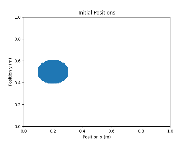
The visualise_particles.{py, ipynb} script generates scatter plots visualising the initial and final positions of particles in an Smoothed Particle Hydrodynamics simulation. The script extracts data from CSV files and uses the simulation boundaries defined in a separate domain file to create informative plots.

The script uses two Python modules; the pandas module to read the position data from the CSV files they are stored in and the matplotlib module to create and display the visualisations of the initial and final positions of the particles.

Output of the visualise_particles.{py, ipynb} scripts: Snapshot of the initial positions of the particles for a droplet case.

Usage:

• Ensure you have the following libraries installed in your Python environment: pandas, matplotlib.
• Run the script from the command line, using the command python visualise_positions.py., or run it as a Jupyter notebook, by executing the notebook cells of the visualise_positions.ipynb file.

Inputs:

• CSV files containing particle position data. These files must have Position_X and Position_Y columns.
• Domain file (domain.txt) specifying the simulation boundaries using keyword-value pairs (e.g., left_wall: 0.0).

Outputs:

Separate scatter plots displaying the initial and final particle positions.

Assumptions:

• The expected CSV file format is consistent with Position_X and Position_Y columns.
• The domain file uses the specified keyword-value format for defining boundaries.

2. Energy Plots

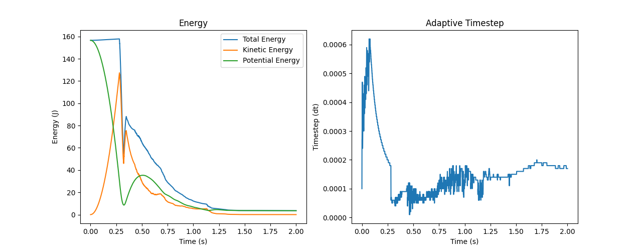
This plot_energies.{py, ipynb} script visualises the total, kinetic, and potential energies of particles throughout an SPH simulation by plotting them against time. Additionally, it plots the evolution of the adaptive timestep used in the simulation over time. The data is extracted from a CSV file containing energy and timestep values at different simulation moments.

The script uses two Python modules; the pandas module to read the energy and timestep data from the generated CSV file and the matplotlib module to create and display the visualisations of all the types of energies measured during the simulation in a single plot.

Output of the plot_energies.{py, ipynb} scripts: Plots of the energy and the timstep evolutions.

Usage:

• Ensure you have the following libraries installed in your Python environment : pandas, matplotlib.
• Run the script from the command line, using the command python plot_energies.py., or run it as a Jupyter notebook, by executing the notebook cells of the plot_energies.ipynb.

Inputs:

• CSV file (energies.csv) containing columns for time (Timestamp), timestep (Timestep), kinetic energy (Ek), potential energy (Ep), and total energy (Etotal).

Outputs:

• Two line plots side-by-side. The left one displays the total, kinetic, and potential energies of particles as functions of time, while the right one displays the adaptive timestep of the simulation over time.

Assumptions:

• The expected CSV file format adheres to the specified column names (Timestamp, Timestep, Ek, Ep, Etotal).

3. Simulation Animation

This simulation_animation.{py, ipynb} script generates an animation visualising the positions and energy evolution of particles, along with the progression of the size of the adaptive timestep used in an SPH simulation across its duration. It dynamically reads data from CSV files containing particle positions and energy and timestep values at different time points of the simulation. The animation depicts both a scatter plot for particle positions and line plots, one for the total, kinetic, and potential energies over time and one for the adaptive timestep.

The script uses two Python modules; the pandas module to read the data from the CSV files they are stored in and the matplotlib module to create and display the dynamic visualisations of the initial and final positions and the energies of the particles.

The number of animation frames is automatically calculated based on the desired_animation_duration, which is automatically calculated based on the simulated time, and the set frame_rate, resulting in a smooth and informative representation of the simulation's progress. This dynamic and adaptable approach ensures the animation effectively captures the key aspects of the SPH simulation for analysis and visualisation purposes.

The code of this script is structured in different functions to provide a concrete separation of concerns for each part of the code.

• get_axes_limits: gets the axes limits for the positions plot from the input domain.txt file
• calculate_num_particles: dynamically determines the number of particles used in the SPH simulation using the generated simulation-positions.csv file. This is required as the number of particles can be potentially different than the one provided by the application user, when it is decided this is needed to properly perform the simulation, such as when the initial condition is set to droplet.
• create_figure: builds the final plot figure that shows the animated position and energy and adaptive timestep data
• update: this function is utilised by the FuncAnimation function of the matplotlib.animation class to update the plot at each frame of the animation
• create_animation: coordinates the creation of the animation of the particles' positions, energies, and adaptive timesteps and stores the generated plot in an MP4 file

Output of the simulation_animation.{py, ipynb} scripts: Animation of the particles' positions, energies and timstep evolutions.

Usage:

• Ensure you have the following libraries installed in your Python environment: pandas, matplotlib.
• Run the script from the command line, using the command python simulation_animation.py., or run it as a Jupyter notebook, by executing the notebook cells of the simulation_animation.ipynb file.

Output:

• An animated MP4 file named fluid_simulation_\<timestamp>.mp4 is saved in the script's directory (i.e. /post/), visualising the SPH simulation dynamics.

Details:

The animation depicts particle positions using scatter plots and tracks their motion through time. Three energy lines represent the total, kinetic, and potential energies of the system throughout the simulation. The animation duration is set based on the simulation time and a configurable frame rate. This script leverages dynamic particle count determination and customisable styles for a versatile animation experience.

Assumptions:

• The expected CSV file formats conform to specified column names (Position_X, Position_Y, Timestamp, Timestep, Ek, Ep, Etotal).
• The number of timesteps is the same between the two files holding the position and energy data, i.e. simulation-positions.csv and energies.csv