Central Tendency
We have seen how data graphics of various kinds can be used to explore the distributions of any variable.

Very often, we want to be able to summarise sampled distributions with a single value that represents a "typical" or "average" value. There are three common ways to calculate this central tendency.
- arithmetic mean, $\bar{x}$
- median
- mode (for discrete or categorical data)
We represent the data as ${x_{1}, x_{2}, x_{3}, ..., x_{n}}$
Arithmetic Mean
Add all the data together and divide by the number of data points, $n$.
$$ \bar{x} = \frac{1}{n}\sum_{i=1}^{n} x_i $$
$\bar{x}$ is the sample mean.
The population mean is given the symbol $\mu$.
The sample mean is used as an estimate of the population mean.

Median
Sort the data by ascending value.
If $n$ is odd, take the value in the middle of the list.
If $n$ is even, take the midpoint of the middle two values.

Mode
The mode is the value that occurs most frequently. There can be more than one mode (if there is a tie).
It is the only measure of central tendency that is applicable to categorical data.
It can also be applied to discrete (or binned continous) numerical data.

Dispersion
In addition to its central tendency, we will usually want to summarise the dispersion of the data, i.e. its degree of variability around the average.
Once again there are several possible statistics to choose from:
- variance, $s^{2}$
- standard deviation, $s$
- inter-quartile range (IQR)
Variance
This is defined as the expectation of the squared deviations of the data from the mean (i.e. the second central moment of the distribution).
$$ m_{2} = E[(X - \mu)^{2}] \approx \frac{1}{n}\sum_{i=1}^{n}(x_i - \bar{x})^{2} $$
This would be the correct definition of variance if we only wanted to describe the data themselves.
Usually though, we want to use this statistic as an estimate of the population variance. The above formula will consistently underestimate this value, and this discrepancy can be important for small sample sizes. We say that the estimate is biased.
To fix this bias, we swap the $1/n$ for $1/(n - 1)$:
$$ s^{2} = \frac{1}{n - 1}\sum_{i=1}^{n}(x_i - \bar{x})^{2} $$
$s^{2}$ is the unbiased estimator for the population variance, usually called the sample variance.
variance of penguins' mass = 643131.077 g^2
Standard Deviation
This is the square root of the variance.
It is usually a more helpful summary, as it is in the same units as the data themselves.
$$ s = \sqrt{ \frac{1}{n - 1}\sum_{i=1}^{n}(x_i - \bar{x})^{2} } $$
Remember that the formula for $s$ using $1/(n - 1)$ instead of $1/n$ is based on the unbiased estimator for the population variance.
We call this the sample standard deviation.

Inter-Quartile Range
The first quartile $Q_{1}$ is the value greater than 25% of the data (i.e. the 25th percentile).
The third quartile $Q_{3}$ is the value greater than 75% of the data (i.e. the 75th percentile).
The inter-quartile range IQR is $Q_{3} - Q_{1}$.

Box Plot
The lower quartile, median and upper quartile are marked in a traditional plot called a box plot, which can give a simple summary for a distribution in a similar way to a violin plot (but with less detail).
The minimum and maximum are shown as the whiskers extending from the box.
However, any data further than 1.5 IQRs away from the box are shown as individual "outlier" points.


Shape of a Distribution
As well as the central tendency and dispersion, we are sometimes interested to characterise the shape of the distribution. There are two commonly used statistics for this purpose:
- skewness, and
- excess kurtosis
Skewness
The skewness tells us how asymmetric the data is. It is defined as
$$ \gamma = \frac{m_{3}}{m_{2}^{3/2}} $$
where
$$ m_{j} \approx \frac{1}{n}\sum_{i = 1}^{n}{(x_{i} - \bar{x})^{j}} $$
is the $j$ th central moment of the data.
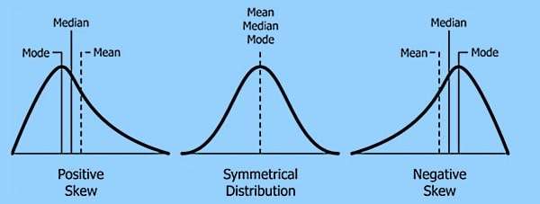
A skewness of zero indicates a symmetrical distribution.
A skewness above zero (positively skewed) means more weight is in the right tail.
A skewness below zero (negatively skewed data) means more weight is in the left tail.

skewness of culmen_length_mm = 0.053
skewness of culmen_depth_mm = -0.143
skewness of flipper_length_mm = 0.344
skewness of body_mass_g = 0.468
When data is substantially skewed, the mean and standard deviation will be strongly affected by the extreme data points. Hence these are no longer truly representative of the dataset as a whole.
For skewed data, the median and the IQR are considered to be better summary statistics, as these are not affected by the extreme values.
Excess kurtosis
The excess kurtosis tells us about the tailedness of the data. It is defined as
$$ \kappa = \frac{m_{4}}{m_{2}^{2}} - 3$$
where
$$ m_{j} \approx \frac{1}{n}\sum_{i = 1}^{n}{(x_{i} - \bar{x})^{j}} $$
is the $j$ th central moment of the data.
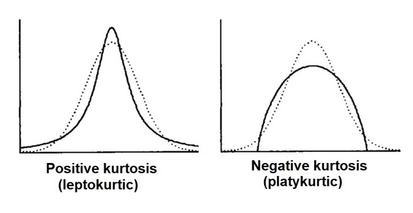
A normal distribution has excess kurtosis of zero.
A value above zero (leptokurtic) means the tails are heavier than a normal distribution.
A value below zero (platykurtic) means the tails are lighter than a normal distribution.
excess kurtosis of culmen_length_mm = -0.881
excess kurtosis of culmen_depth_mm = -0.911
excess kurtosis of flipper_length_mm = -0.987
excess kurtosis of body_mass_g = -0.726
Correlation between Two Variables
We often want to measure the strength and direction of an association between two variables. There are two common measures of this correlation:
- Pearson product moment correlation coefficient
- Spearman rank correlation coefficient
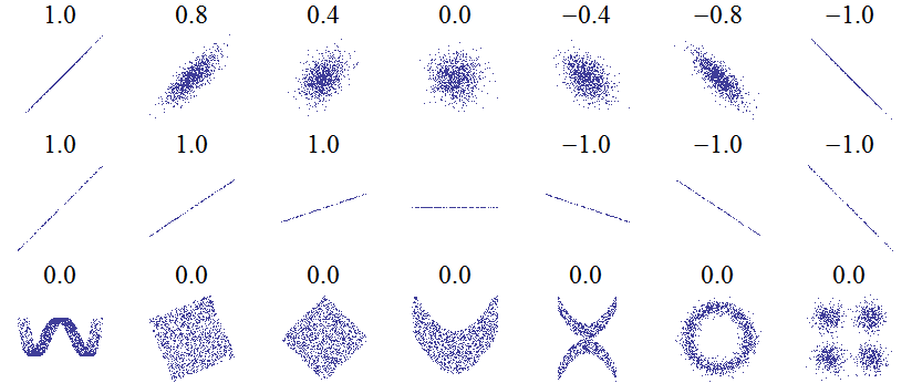
Pearson Product Moment Correlation Coefficient
This is a measure of linear correlation - to what extent do the data resemble a straight line with an increasing or decreasing slope?
$$ r_{x,y} = \frac{\sum{x}_{i}{y}_{i} - n\bar{x}\bar{y}}{(n - 1)s_{x}s_{y}} $$
This value is bounded at +1 (perfect correlation) and -1 (perfect anticorrelation).

| flipper_length_mm | body_mass_g | |
|---|---|---|
| flipper_length_mm | 1.000000 | 0.871202 |
| body_mass_g | 0.871202 | 1.000000 |
pearson correlation of flipper_length_mm with body_mass_g = 0.871
Spearman's Rank Correlation Coefficient
Because Pearson's measure of correlation assumes a linear relationship between the variables, it does not give useful results when the association is far from linear.
Spearman's version uses the same formula, but works with the ranks of the data instead of their values.
$$ \rho = r(R[X],R[Y]) $$
where e.g. $R[(3.4, 5.1, 2.6, 7.3)]$ is $(2, 3, 1, 4)$

Pearson correlation =  0.864
Spearman correlation = 1.0

Pearson correlation of Length with Weight = 0.925
Spearman correlation of Length with Weight = 0.973
Limitations of Summary Statistics
We cannot rely on summary statistics alone to fully describe data distributions or the relationships between variables. This is why data visualisation is so important in being able to understand our data properly.
Anscombe's quartet is a set of four datasets that illustrates this point.

DATASET  I :
mean x = 9.0
sd x = 3.1622776601683795
mean y = 7.500909090909093
sd y = 1.937024215108669
Pearson correlation (x, y) = 0.8164205163448399

DATASET  II :
mean x = 9.0
sd x = 3.1622776601683795
mean y = 7.50090909090909
sd y = 1.93710869148962
Pearson correlation (x, y) = 0.8162365060002427

DATASET  III :
mean x = 9.0
sd x = 3.1622776601683795
mean y = 7.5
sd y = 1.9359329439927313
Pearson correlation (x, y) = 0.8162867394895984

DATASET  IV :
mean x = 9.0
sd x = 3.1622776601683795
mean y = 7.500909090909091
sd y = 1.9360806451340837
Pearson correlation (x, y) = 0.8165214368885028