|
ICFERST
25-11
Reservoir simulator based on DCVFEM, Dynamic Mesh optimisation and Surface-based modelling
|
|
ICFERST
25-11
Reservoir simulator based on DCVFEM, Dynamic Mesh optimisation and Surface-based modelling
|
(This text is in manual.F90)
All the contributions to ICFERST in this repository are under AGPL 3.0 license, otherwise refrain from commiting your code to this repository. Each library keeps their original license.
The executable is named icferst
The schema for the ICFERST diamond interface is in ICFERST/schemas/multiphase.rmg
For compilation run the command from the root folder:
./configure --enable-2d-adaptivity && make mp!>
ICFERST is property of the NORMS group. See the file COPYRIGHT for a description of the copyright.
For more details please see: http://multifluids.github.io/ or http://www.imperial.ac.uk/earth-science/research/research-groups/norms/
1) Download it from github with the following one-line command
git clone https://github.com/ImperialCollegeLondon/multifluids_icferst.git
2) Install dependencies
 sudo apt-add-repository ppa:fluidity-core/ppa
 sudo apt-get update
 sudo apt-get install fluidity-dev autoconf-archive python-is-python3 pkg-config
3a) Ubuntu 18.04, modify the .bashrc file in home to include
export PETSC_DIR=/usr/lib/petscdir/3.8.3
3b) Ubuntu 20.04, modify the .bashrc file in home to include
export FCFLAGS="-I/usr/include"
3c) Ubuntu 24.04, set up the configuration file correctly by running
autoreconf --force --install
3d) You may need to explicitly include the python dependencies
export PYTHONPATH=/usr/lib/python3
4) Navigate to the root directory of your ICFERST folder. You can install the application for all users by running:
 cd IC-FERST-FOLDER/
 ./configure --enable-2d-adaptivity
 make mp && sudo make install
Or you can install it locally (only for your user) by running:
 cd IC-FERST-FOLDER/
 ./configure --enable-2d-adaptivity --prefix=$HOME/ICFERST
 make mp && make install
Within the folder ICFERST/tools you can find some useful scripts:
1) If detectors are used you can use detectors_and_stat2csv.py to convert the detectors file in the more readable format .csv
2) To convert from Cubit (exodusII) to a mesh type that ICFERST can open (GMSHv2 format) the scripts exodus2gmsh.py (3D) and 2Dexodus2gmsh.py (2D can be used. exodus2gmsh.py can convert directly into binary format
3) Within scripts_to_make_life_easier there are two scripts to be modified and copied (manually) into /usr/bin to make the use of Diamond and ICFERST much easier.
The formulation of the IC-FERST code is split in:
1) The manual in ICFERST/doc which is outdated but contains a very detailed description of the mathematical formulation
2) Papers published containing the formulation used in IC-FERST:
For more information of each specific method a link to the corresponding paper has been added in each section within Diamond interface
IC-FERST uses PETSc to access a set of linear solvers to solve the systems of equations. The method is the typical one where a Krylov subspace method (typically GMRES due to its robustness and flexibility) is used to solve the linear system of equations using a preconditioner based on on an algebraic multigrid method to ensure a fast convergence.
GMRES works by approximating the solution by the vector in a Krylov subspace with minimal residual and iterating until the solution with the desired quality is achieved. For GMRES, the speed of the convergence heavily relies on the conditioning number of the system to be solved for. Moreover, GMRES convergence depends on the number of degrees of freedom to be solved for. In this way, the use of a preconditioner is used to accelerate the process. Among all the possible accelerators (preconditioners), the fastest and the only one whose convergence is independent of the number of degrees of freedom is multigrid. Other can be used, such as Jacobi or ILU, but its convergence degrades as the number of degrees of freedom increases.
Multigrid works by eliminating the high frequencies of the error using a smoother (typically performing a couple of Jacobi or Gauss-Seidel iterations) and then moving the residual to a coarser mesh, where the process is repeated and its result is used to improve the result of the finer mesh. This process is recursive and therefore a set of levels can be used, and therefore, a multigrid method is obtained. Due to its nature, multigrid convergence is independent on the degrees of freedom. However, elaborate operators need to be tailored for specific system of equations and meshes to obtain an optimal performance. In ICFERST the use of HYPRE as preconditioner when using the DCVFEM shows excellent performance and it is the recommended (and default choice).
In the previous section we have discussed the use of GMRES and multigrid. These solvers can solve only linear systems of equations (although multigrid with the Full Approximation Scheme can also solve non-linear system of equations by including the Newton-Raphson method as part of the smoother). Therefore we also require a non-linear solver to deal with the non-linearities arising when solving the full system of equations. Non-linearities may arise from Equations of State, relative permeability, capillary pressure, dependence with other fields (for example transport depending on temperature), etc.
The typical approach to solve a non-linear system of equations is the use of a fixed-point iterative method. A Fixed-point iterative method, as its name says, pivots around a fixed-point to identify a "direction" to follow in order to obtain the solution. The most famous ones are: i) Newton-Raphson: the direction of the gradient is used to find the solution. If the solution field is continuous the convergence is quadratic. This method requires to generate a Jacobian matrix and tends to generate bigger and harder matrices to solve for than the alternative. ii) Anderson solver: In this case the system is linearised by freezing all the fields that are not part of the current linear solve. For example if solving for pressure then all the other fields are constant at that stage. By iterating through the different linear systems, the non-linear system is finally solved. This approach has typically a first order convergence but in exchange the systems to solve for are easier and smaller.
In both cases and as described so far, the non-linear solvers have only "local" convergence, meaning that the initial guess of the solution needs to be relatively close to the final solution for the solver to be able to solve for it. Otherwise the solver will typically diverge, or find a local optimal, obtaining wrong result. To increase the range of convergence to "global" convergence (note that no non-linear solver has really global convergence as it cannot be guaranteed so the term is used to describe a wider range than just local convergence) several methods have been developed, backtracking, trust region, double dogleg, just to mention some. In all these methods, the idea is to correct the prediction to ensure that the solver does not overshoot and also, to try to avoid local minima. In ICFERST a backtracking method with acceleration is currently implemented to do both, improve the convergence and stability of an Anderson solver.
All the ICFERST code is within the folder ICFERST where the test cases, code, tools and schemas for diamond are stored. Some parts of Fluidity have been slightly modified but in general the Fluidity code is untouched. ICFERST is composed of two main loops. First, it is the time loop and secondly the non-linear loop, which is a Picard method to deal with non-linearities. The time-loop is defined in the multi_timeloop file. From this subroutine we initialise all the necessary fields and start the non-linear loop, within which all the equations to be solved are being called as blocks. In this way, first the momentum equation and velocity are obtained, next the saturation is transported (which also contains within it another non-linear loop) and then all the other transport equations are being solved.
ICFERST solves the system of equations using a DCVFE formulation, which means that we use two different meshes, a CV mesh and a FE mesh. The CV mesh and associated equations are dealt with in CV_ASSEMB, which for porous media is around 70% of the overall cost. Everything related with the FE mesh is solved for in multi_dyncore However multi_dyncore contains the calls to solve for the different transport equations. So effectively the process is normally time_loop (initialise memory and stuff, including EOS, source terms...) => multi_dyncore (assemble and solve) => cv_assemb (assembles the transport equation).
To simplify and standardize the naming of the variables the structures defined in multi_data_types are used through the code. Normally one or two of those types are created once and used throughout the code, so it is recommended to check in that section what is each variable and use those types either expanding them or creating more.
     ┌─────────────┐     ┌────────────┐    ┌───────────────┐
     │Adapt_state  ├─────┤Adaptivity  ├────┤ Mesh2Mesh int │
     └─────────────┘     │ (assemble) │    └───────────────┘
                         └─────┬──────┘
                               │          ┌────────┐
                               │   ┌──────┤  PETSc │
                               │   │      └────────┘
       ┌─────────────┐   ┌─────┴───┴─┐    ┌───────────────────┐
       │ Read input  ├───┤ Fluidity  ├────┤ Generate vtu files│
       └─────────────┘   │ (femtools)│    │  detectors, stats │
                         └──────┬────┘    └───────────────────┘
        ┌──────────────┐        │                        ┌────────────────────────────────────────────────────┐
        │Populate_state├────────┤                        │multi_phreeqc──────────►Initialise PHREEQCRM        │
        └──────────────┘        │                        │Shape functions────────►CV and FE shape functions   │
                         ┌──────┴─────┐                  │                                                    │
                         │  ICFERST   │ Initialisation   │Multi_data_types ──────►Initialise types and memory │
    ┌───────────────────►│  Timeloop  ├─────────────────►│                                                    │
    │                    │            │  of after adapt  │multi_eos  ───────────► Update EOS and petrophysical│
    │                    └──────┬─────┘                  │                        properties                  │
    │                           │Start non-linear        │Extract from state ────►Read from diamond and       │
    │        ┌─────────────────►│ loop                   │                        adaptive-time-stepping      │
    │        │                  │                        └────────────────────────────────────────────────────┘
    │        │           ┌──────┴───────────┐
    │        │           │Assemble and solve│      ┌───────────────────┐  ┌───────────┐ ┌───────────────────┐
    │        │           │momentum equation ├─────►│  multi_dyncore    ├─►│ cv_assemb ├─► Assemble C and Ct │
    │        │           └──────┬───────────┘      └─┬─────────────────┘  └───────────┘ └───────────────────┘
    │        │                  │                    │    ┌───────────┐
    │        │                  │                    ├───►│Assemble M │
    │        │                  │                    │    ├───────────┴────────────┐     ┌────────────┐
    │        │                  │                    │    │ Solve  (M  C) (u) = (f)├────►│multi_solver│
┌───┴─────┐  │      ┌──────────►│                    └───►│        (Ct Mp)(p)   (g)│     └────────────┘
│ Advance │  │      │           │                         │ Mp/=0 for compressible │
│  time   │  │      │   ┌───────┴────────────┐            └────────────────────────┘
└───┬─────┘  │      │   │If multiphase solve │     ┌─────────────┐        ┌─────────┐   ┌───────────┐
    │        │      │   │transport saturation├────►│multi_dyncore├───────►│cv_assemb│──►│multi_pipes│
    │        │      │   └────────┬───────────┘     └─────┬───────┤        └─────────┘   └───────────┘
    │        │      │ Loop until │                       │  ┌─────────────────────────────┐
    │        │      │ converge   │                       └──┤ solve and backtrack solution│
    │        │      └────────────┤                          └─────────────────────────────┘
    │   ┌────┴───────────┐       │                 ┌─────────────┐
    │   │ Adapt time-step│       │                 │Temperature  ├───────┐
    │   │   size         │       │                 ├─────────────┤       │  ┌─────────────┐  ┌─────────┐   ┌───────────┐
    │   └────┬───────────┘       │                 │Concentration├───────┼─►│multi_dyncore├──►cv_assemb│──►│multi_pipes│
    │        │                   │───────────────► ├─────────────┴───────┤  └────┬────────┘  └─────────┘   └───────────┘
    │        │                   │                 │ActiveTracers/Species├──┐    │   ┌────────────┐
    │        │ Loop until        │                 ├─────────────┬───────┤  │    └──►│solve system│
    │        │ convergence       │                 │Compositional├───────┴──┤        └────────────┘ ┌─────────────────────────┐
    │        └───────────────────┤                 └─────────────┘          └──────────────────────►│PHREEQC Update Species   │
    │                            │                                                                  └─────────────────────────┘
    │                            │       ┌──────────────┐       ┌──────────────┐   ┌─────────┐   ┌───────────┐
    │                            ├──────►│PassiveTracers├───────►multi_dyncore ├──►│cv_assemb│──►│multi_pipes│
    │                            │       └──────────────┘       └┬─────────────┘   └─────────┘   └───────────┘
    │                            ├─────────────┐                 │  ┌────────────┐
    │                    ┌───────┴──────────┐  │                 └─►│solve system│
    │                    │  Output vtu      │  │                    └────────────┘
    │                    │         outfluxes│  │
    │                    └───────┬──────────┘  │   ┌──────────────┐
    │                            │             └──►│SelfPotential │
    │                     ┌──────┴────┐            └──────────────┘
    │                     │ Adapt mesh│
    │                     └──────┬────┘
    └────────────────────────────│
                              ┌──┴──┐
                              │ END │
                              └─────┘
ICFERST uses two types of structures which are effectively linked lists pointing to either scalar_fields, vector_fields or tensor_fields. The first field is state, which is an array containing as many entries as phases. Within each entry one has all the fields defined in diamond. These fields are the ones that Fluidity "see" and therefore will perform its operations on it, such as computation of statistics of the field in the .stat file, output it into the .vtu file, perform mesh to mesh interpolation, etc. To access these fields one has to do as follows to extract a scalar field:
sfield=>extract_scalar_field(state(iphase),"Density")
it can be seen that we use the command extract_scalar_field (substitute scalar by vector or tensor depending on the field), then we use its name and we use a type(scalar_field), pointer to point to the memory provided by the function extract_scalar_field. #For more information about scalar_fields, etc. please see the Fluidity manual. As summary, these fields contain its value as sfieldval with as many entries as the ones on the mesh in which the field was initialised. Common fields are: Pressure, Velocity, PhaseVolumeFraction, Temperature and Concentration.
The second field is packed_state. Packed_state contains the same fields as state (at least the prognostic ones) and the memory is actually shared. packed_state however contains the fields as (normally) tensor_fields so all the phases can be accessed naturally. For example for PhaseVolumeFraction we would do as follows:
tfield=>extract_tensor_field(packed_state,"PackedPhaseVolumeFraction")
note that now we are using a tensor_field, we used Packed before the name of the field and packed_state is not an array. The obtained field would have the following entries: tfieldval(ncomp,nphase,CV_nonods), normally ncomp == 1. For velocity it would be: tfieldval(ndim,nphase,CV_nonods).
ICFERST is a dimension agnostic code and therefore it is FUNDAMENTAL that the units used, unless otherwise specified, are the S.I. units to ensure consistency on the results obtained.
The procedure to use IC-FERST is the following:
Generate a model and a mesh => Set up the physics of the model with diamond => Run ICFERST => Examine outputs with Paraview
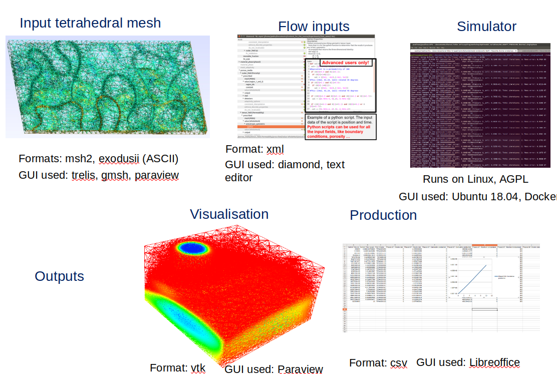
IC-FERST can currently only read .msh files following the format described by GMSHv2 or GMSHv4. For a model to work with IC-FERST it must be meshed with either triangles in 2D or tetrahedra in 3D. Boundaries must be specified with surface ids and the different material properties must be defined with region IDs following the Surface Based modeling paradigm. Although only the GMSH files can be read, normally Cubit is used to generate the models as it is more powerful and the files exported in ExodusII can easily be converted to GMSHv2 format using the scripts described in Useful scripts
To model wells, it is necessary to define a line that describe the well path. As ICFERST cannot respect 1D lines when adapting the mesh, normally this is achieved by generating a well-sleeve composed of three regions whose central connection represents the well path. In this way we ensure that mesh adaptivity will respect the well path and also ensures a minimum precision around the well. To provide the well path to ICFERST there are two alternatives:
1) Generate a nastran (.bdf) file per well describing the well path with nodes and edges.
2) If the well is a straight line then only by defining the top and bottom coordinates are enough.
Under the section /porous_media/wells_and_pipes the user can find all the required fields that can be modified to set up a simulation with wells. The wells consider a modified Darcy equation to model flow within the pipes, meaning that we are solving the flow within the pipe. To set up a well the user must define:
Currently, ICFERST model wells by considering that two different domains co-exist and are connected through the nodes of the wells. To define this through diamond, one has to duplicate the number of phases to the ones required to model the system without wells and consider that they are equivalent, for example for two phase phase 1 and 3 are the same. Therefore, the EOS and different properties must be defined equivalently. Another important requirement is that now two Pressure needs to be solved for, in this case phase 1 and 3 will have a defined pressure and phase 2 and 4 will be aliased with 1 and 3 respectively. Once this is done the boundary conditions need to be set accordingly
ICFERST can use XGBoost to accelerate the non-linear solver using a pre-trained model based on dimensionless parameters (Silva et al. 2022). In order to activate this option XGBoost needs to be installed and liked with ICFERST, this latter can be done with the following command:
and then specify the model path in /solver_options/Non_Linear_Solver/Fixed_Point_Iteration/ML_model_path
./configure --with-xgboost && make mp
Since currently the model is very heavy, it takes 2GBs, the model is not stored online so currently it needs to be requested to ICFERST developers.
Using the diamond GUI to configure test cases The input files are “EXAMPLE.mpml”. This files can be either manipulated using diamond a GUI, or a text file. To open the diamond GUI for ICFERST this is an example, found in the examples folder in IC-FERST-FOLDER/legacy_reservoir_prototype/tests/3D_BL_P0DGP1CV
IC-FERST-FOLDER/libspud/diamond/bin/diamond -s IC-FERST-FOLDER/ICFERST/schemas/multiphase.rng 3D_test.mpml
Diamond requires a file predefining the entries to be created and that can therefore be modified by the user. This is done using a schema. The schema for ICFERST is stored in ICFERST/schema. Here the main file is multiphase.rnc which calls the other ones as required. Note that there are two files, the .rnc and the .rng. The .rnc file is to be modified by a developer and then compiled using the tool spud-preprocess. The .rnc file uses a hierarchical language with different operators to define whether reals, integers or booleans are required as inputs, as well as different options for the settings. It is recommended to expand the .rnc file based on pre-existing examples within the .rnc file.
To add/remove or modify the schema the .rnc files need to be modified as required and afterwards recompiled using spud-preprocess:
this will generate new .rng files which are the ones read by diamond. spud-preprocess should have been installed in your system as part of the make install process.
spud-preprocess multiphase.rnc
You can find a tutorial detailing the use of diamond and the different sections in ICFERST/doc/ICFERST_tutorial.pdf (Like the figure below)
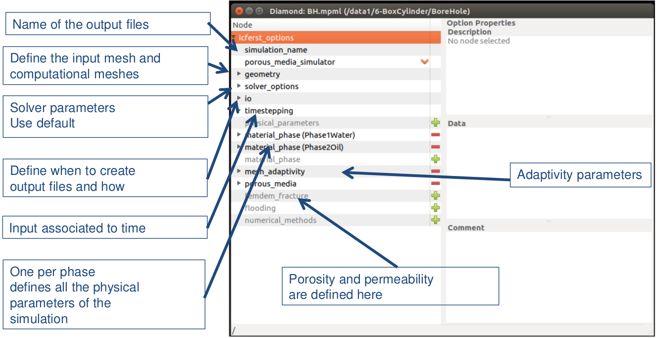
Here we will provide a short summary of each section but the graphical document is still highly recommended, also more information of each field is already in place in the Diamond interface itself in the description box.
In this section the user must define the dimensions of the mode, the input file and the simulation quality. Currently only Fast and Balance are operative the other settings are just for research purposes and its use is not recommended. The option create_binary_mesh is used to convert the given mesh into a binary format to be used by fldecomp, if this option is one the recommended usage is to use it and kill the simulation once the conversion has been done (printed on the terminal).
This zone is devoted to modify the linear and non-linear solvers. It is recommended not to modify the linear solver settings unless a model with undefined pressure is used, in which case the pressure solver needs to be defined with the option remove null space. Even for this cases it is recommended to use the default settings of GMRES(30)+Hypre and relative residual reduction of 1e-10
Regarding the non-linear solver settings, it is also recommended not to modify it unless the adaptive time-stepping method with PID is used in which case the user is encouraged to introduce the defaults settings for all the requested fields and specify the PID adaptive time-stepping.
The recommended method to adjust the time-step size in ICFERST is to do it based on the stability of the non-linear solver with the addition of the PID controller (Proportional Integrator Derivation). Adaptive time-stepping methods based on the stability of the non-linear solver normally suffer from the fact that they keep raising the time-step size until they fail, which forces them to repeat a time-level, halve the time-step size and repeat the process. This is suboptimal. In ICFERST, we use a PID type method based on a requested number of non-linear iterations, where the controller adjusts the time-step size to try to always have the same number of non-linear iterations, avoiding that problem and being overall more efficient.
For more information see: link Hamzeloo et al 2022.
The Vanishing Artificial Diffusion (VAD) is devoted to stabilise the system when solving for multiphase flow. It can also be used for transport however we have seen that in certain scenarios it may not be beneficial, this could be solved adjusting the parameter but this work needs to be done. However, for multiphase it has shown to greatly accelerate the non-linear solver and specially when having capillary pressure in the system. Unless explicitly imposed, when capillary pressure is active VAD is also active. Moreover, VAD is active if no settings of the non-linear solver are set.
Recentely, it has been observed that for big density ratio between the phases it can lead to mass generation. Therefore it is advised to disable it (set to zero) when the density between the phases is more than one order of magnitude.
For more information see: link Salinas et al 2019.
The momentum_matrix settings are only for stokes and therefore out of the scope of this manual.
In this section the user can specify what to output from ICFERST. The outputs of vtu files can either be based on timesteps or time in seconds. The user can select to:
The initial time, final time and initial time-step size is selected here. Also a time-stepping method based on a CFL limit can be specified here. Note that if the time-step is to be adjusted on both the CFL and the non-linear solver, the most limiting one will be used.
The user can select the magnitude and direction of the gravity forces as well as select from two options to help with hydrostatic modelling hydrostatic pressure solver, which requires an extra solver and does not work with Wells or remove hydrostatic contribution, only for single phase.
You can add as many phases as desired in theory, however ICFERST can only do up to three phases (gas, liquid, aqua), doubling to 6 if having wells. It is important to note that pressure is only solved for the first phase and the other phases are aliased with this phase. Within each phase the user has to defined its viscosity and different properties based on the modelling requested. PhaseVolumeFraction has to be always defined even though a single phase model is done.
A phase must have a pressure field defined, a Velocity field and a PhaseVolumeFraction defined. Also, temperature, concentration and Passive/ActiveTracers can be defined as well as species. To define a Passive/ActiveTracer the fiel must start with that name, for example ActiveTracer_Humidity. In this way, n-fields can be solved for. There are some more restricted fields or diagnostic fields that are used by Fluidity that the user can take advantage of, we recommend the reader to check the Fluidity manual for those.
For multiphase, the section multiphase_properties must be defined. There the relative permeability, immobile fraction and capillary pressure can be defined.
ICFERST accepts three types of BCs all of them weakly enforced (excepting pressure dirichlet for wells): Dirichlet, zero_flux and Robin. If Neumann are required the recommendation is to use Robin without the dirichlet contribution.
The minmax principle states that without sources or sinks a field is bounded between its initial value and boundary condition values. Providing this information when possible ensure first that the results obtain are going to be physically possible (if not specified the concentration could accumulate in a certain CV endlessly!) and also helps the non-linear solver to achieve convergence faster by constraining the area of search. For tracer fields, it is HIGHLY recommended to specify the min_max condition since it helps ensure a physical solution as well as accelerate the simulation.
ICFERST uses a-priori error estimation method based on Cea's lemma. Therefore, it is possible to adjust the mesh to minimise the requested error. In this part, the user can specify the desired precision of the field. If using absolute this is with the same units, for example 1000 for pressure would be that the user wants a precision of 1KPa in the results, below this the mesh won't capture it. The relative option does the same but considering the bounds of the field dynamically, some users have experienced problems with relative and therefore absolute is recommended.
Once a new mesh is generated the fields need to be interpolated between meshes. Interpolation between meshes needs to take into account: i) Conservation: the integral of the field before and after is the same, ii) Boundedness: the maximum and minimum values before and after the interpolation are the same iii) artificial diffusion: does the interpolator introduces artificial diffusion into the solution? Within ICFERST, The Galerkin projection fulfils all three but it is expensive as a system of equations needs to be solved for. Consistent interpolation fulfils ii) and iii) and Grandy fulfils i) and ii) but not iii). In this way it is recommended to use Galerkin for scalar fields and velocity and consistent interpolation for wells and pressure.
A source term can be added to every field. The absorption term however is inactive. Only defining a tensor field named UAbsorB on the first phase this can be used. UAbsorB can be used to modify the momentum equation through the diamond interface.
To activate mesh adaptivity there are two different parts. The user first needs to select the type of interpolation and specify the precision requested for the fields of interest using Adaptivity options and Mesh to Mesh interpolator and secondly activate the settings in mesh_adaptivity/hr_adaptivity
Within this section the user can select
Other settings to take into account are adapt at the first time step, which can be used to generate a mesh from a given one or if there is an interface at the beginning. The fail safe is on by default and it is not recommended to modify it, similar to the other settings.
In this part the user must specify the petrophysical properties under porosity, permeability, and if needed, Dispersion and rock properties such as density, heat capacity and coductivity of the porous media under porous properties.
Under thermal well properties the user can also define the conductivity of the pipe and its thickness so the pipes can also interchange heat where they are close to flow
-Well volume ids: The user must specify here the sleeves conforming the well path. If selected lock sleeve nodes, then DMO will lock the nodes within these regions, ensuring that the result is less oscillatory (although perfectly correct anyway).
Well from coordinates: alternatively if the well is a straight line, you can specify it just using coordinates.
IC-FERST can run reaction modelling where the reaction part is performed using PHREEQC. To do this first the user must install PHREEQCRM on the system and compile IC-FERST to support this with the following command:
Next, a PHREEQC file needs to be generated as normal and provided it through the command /porous_media/Phreeqc_coupling/simulation_name.
./configure --with-phreeqc && make mp
By activating /porous_media/SelfPotential that computation will be performed. Some extra parameters are required, which can either use the default ones or use the python interface from python to introduce different models.
It is very important to define a reference coordinate where the Voltage will be set to zero, and everything in reference to that. Moreover, if not temperature field is solved for, a reservoir temperature needs to be provided. For more information of the default models read Mutlaq et al. 2020.
IC-FERST can model instantaneous gas dissolution into a fluid using this option and as a flash calculation that occurs after the non-linear solver.
Diamond enables the user to introduce Boundary Conditions and diagnostic fields, as well as other fields such as SelfPotential parameters using python code. It is important to note that using a python field is considerably slower than using a field based on region ids, this extra cost is not unbearable but it is neither negligible. Therefore, the use of python fields is only recommended only if strictly necessary.
For boundary conditions and simple fields, the python code looks as follow to set up Velocity Boundary Conditions based on time:
  # Function code
  def val(X, t):
   import numpy as np
   alpha = 2.5 #m/s - max velocity
   f     = 20./60. #20 breath/min
   angle = np.radians(30.)
   v_ejecta = alpha*np.sin(2.*np.pi*f*t)

   if v_ejecta < 0.:
     u = 0.0
   else:
     u = v_ejecta  * np.cos(angle)

   return u # Return value
it can be seen that it can load modules. This code will be called and evaluated for every single node in the boundary and the only inputs are Coordinates (X) and time (t).
Using diagnostic fields the user can have access to all the fields stored in state (or packed_state, check the description) which enables the user to perform more complex operations such as alter fields. In this way the python call is performed only once per non-linear loop. It is important to note that the python code is parallel safe as long as everything is keep in memory, i.e. not trying to read a file. More information can be found in the Fluidity manual, Appendix B. Here a summary of that content is provided: Basic commands to manipulate scalar, vector or tensor fields:
 import numpy as np

 C = state.scalar_fields['PassiveTracer_H2O']
 P = 1.01325e+5

 T  = state.scalar_fields['Temperature']
 UV = 0.0
 Ref_temp = 20.615+273.15

 for nodeID in range(field.node_count):
   #Convert to relative humidity
   RH=0.263*P*C.node_val(nodeID)*1./(np.exp((17.67*(T.node_val(nodeID)-273.15))/(T.node_val(nodeID)-29.65)))
   k_inf = (0.16030+0.04018*((T.node_val(nodeID)-Ref_temp)/10.585)+0.02176*((RH-45.235)/28.665)+0.14369*((UV-0.95)/0.95)+0.02636*((T.node_val(nodeID)-Ref_temp)/10.585)*((UV-0.95)/0.95))/60.0
   field.set(nodeID, k_inf)
it can be seen how fields can be extracted from state and then looped over them. Compared to the previous script here we need to use commands such as set to impose the value of the field. This approach is very powerful. To include new fields in diamond that can use this it is recommended to link it using multi_compute_python_field following the procedure done for the SelfPotential fields. For more details of available commands check Fluidity's manual. The current version of the multiphase schema found within ICFERST/schemas is a simplified version which gets populated internally so it is compatible with Fluidity. This extra population affects when generating checkpoint files that will not be exactly like the original and may need to amended before re-running from a checkpoint (which can be done by opening them and saving). It is important to understand that this conversion exists since it may affect some sections of the code. However, this has been tried to be kept to a minimum and developers can expect a direct connection between diamond and where the option can be found when extracting it.
The simplification mainly focuses on not having to describe the discretisation type, use of defaults for solvers and other settings , density not being defined as a scalar field explicitly, simplified interpolation settings, etc. These can be found in multiphase_prototype_wrapper and are generated using the spud options as defined in the Fluidity manual in the manual folder
Once you are happy with the contents of your input .mpml file, you can run IC-FERST using:
mpirun -n 1 IC-FERST-FOLDER/bin/icferst 3D_test.mpml
ICFERST can currently be used to model inertia dominated flows (Navier-Stokes), Stokes flow or Darcy flow. This latter is the most commonly used and the main application of ICFERST and therefore this documentation will focus on it. ICFERST can model single (aquifer thermal energy storage) and multiphase flow with or without wells, compositional with reaction provided by PHREEQC (needs to be installed separately).
The recommended action when generating a new simulation is to build from an input file that has the initial settings that you want. There are examples in ICFERST/test/:
All the test cases are run using Github actions every time a commit is done to master or one of the designated branches defined in the file .github/workflows/ubuntu.yml
There are two type of test cases. Ones based on a python script comparing against an analytical solution, or the ones based on checking against data obtained from the .stat file (i.e. min/max of fields, integral etc). In all the cases the test is triggered through the xml file and can be tested locally by running the python script in ICFERST/tools testharness_ICFERST.py The most common flags are -n <#CPUs> and -t <TAG_of_test_cases>. An example of running locally the quick test cases would be:
python3 testharness_ICFERST.py -n 2 -t tbc
For every functionality there MUST be a test case checking that functionality, uniquely if possible.
ICFERST uses openMPI to run in parallel. The mesh needs to be decomposed initially using the command
where #CPUs is the number of CPUs and INPUT_MESH is a binary msh file using the gmshv2 format. This can be obtained using ICFERST from an option in diamond/geometry or from an exodusII file using the python converter from ICFERST/tools Once the mesh is decomposed you can run in parallel using mpirun:
fldecomp -n #CPUs INPUT_MESH
mpirun -n #CPUs icferst INPUT_mpml
where INPUT is INPUT_mpml is the mpml file as normally done. As a rule of thumb one wants to have around 15k elements per CPU to have optimal performance.
 1.8.17